U-2 OS human osteosarcoma cells (ATCC, cat# HTB-96, Manassas, VA) frozen at P4 (2 × 106 cells/vial) were thawed prior to each experiment and were exposed to chemicals within three passages. Cells were cultured in a T75 flask (Corning) in 20 mL of McCoy’s modified 5a medium (ATCC; 30–2007), as per ATCC’s recommendation, supplemented with 10% v/v fetal bovine serum (Gibco) and 1% penicillin–streptomycin (Gibco) at 37 ℃ in 5% CO2. We note that this is different from the Nyffeler et al. (2020) study, which used Dulbecco’s modified Eagle medium (DMEM). Cell density was maintained below 80–90% confluence. To passage the cells, cells were washed in 1 × phosphate-buffered saline solution prior to trypsinization with 0.25% trypsin (Gibco) for up to 5 min at 37 ℃. Cells were suspended in 9 × volume of the maintenance medium to deactivate trypsin. An aliquot (~ 100 µL) of the suspension was collected for Trypan blue staining and counting using an automated cell counter (Countess 3, Invitrogen) and seeded in a T75 flask (maintaining 1 × 105 – 1 × 106 cells/mL) or in 96-well plates (PhenoPlate 96-well microplates, Revvity) 24 h prior to chemical exposures. In 96-well plates, cells were seeded at a density of 5000 cells/well in 100 µL of media using a manual 12-channel pipette.

HTPP reference compounds (Nyffeler et al. 2020) (Table 1) were dissolved in cell culture grade dimethyl sulfoxide (DMSO) (ATCC) to prepare stock solutions at varying concentrations. Treatment solutions were prepared in sterile 96-well plates at 200 × treatment concentration in DMSO. Following the top concentration, the subsequent seven concentrations were spaced by a half-log unit. In a sterile deep-well 96-well plate, 350 µL of exposure media was prepared for each concentration of each reference chemical by adding the treatment solutions to the media at 0.5% v/v. Vehicle controls were prepared with DMSO at a concentration of 0.5% v/v in the media. To expose the cells, the media in the 96-well plate containing the cells was removed and replaced with exposure media prepared in deep-well plates using a 12-channel pipette. Cells were exposed for 24 h. Exposures were performed four times in four independent experiments, where P4 vials of U-2 OS cells were thawed and cultured for each experiment. Each experiment included four 96-well plates, each containing eight DMSO-treated wells (vehicle control), eight concentrations of sorbitol (phenotypic negative control), eight concentrations of staurosporine (cytotoxic control), and eight concentrations of three test chemicals in triplicate. Supplementary Fig. 1 illustrates the plate layout. Well positions were arranged in a fixed order rather than randomized. The highest concentration of each test chemical was placed in row A, with the subsequent concentrations in rows B to H in a decreasing order. Replicates of each concentration were placed in adjacent wells. Experiments 1–3 were identical, containing all 14 chemicals listed in Table 1. Experiment 4 contained amperozide, berberine chloride, fluphenazine, NPPB, and tetrandrine, in addition to the two controls, staurosporine and sorbitol.

In addition, one 96-well plate of cells was treated with 0.5% v/v DMSO only to examine variations in cell count and background variability in phenotypic changes with exposure to DMSO across the wells.

Liquid handling in 96-well plates was performed manually using a 12-channel pipette unless otherwise specified. U-2 OS cells were fixed in paraformaldehyde and stained per the protocol described by Cimini et al. (2023). The volumes were adjusted for 96-well plates. The concentrations of the fluorescent dyes in the wells were consistent with those reported by Cimini et al. (2023). These concentrations differ from the concentrations used by Nyffeler et al. (2020), which were higher for all dyes, except for MitoTracker Red. We conducted pilot experiments (data not shown) using the Cimini et al. (2023) concentrations to conserve dyes and retained these concentrations for the definitive study after confirming the high quality of the resulting images.

Briefly, all dyes were solubilized in their respective solvents to prepare stock solutions at concentrations specified in Table 2. After 24 h of chemical exposure, approximately 50% of the exposure media (45 µL) was removed from each well and replaced with 27 µL of MitoTracker Red working solution (final concentration of 0.5 µM in the well) and the cells were incubated at 37 °C for 30 min. Cells were fixed by adding 27 µL of 16% paraformaldehyde aqueous solution (Electron Microscopy Sciences; cat# 15,710) to each well (approximately 4% final concentration in the well) and incubating at room temperature for 20 min in the dark. Using an automated plate washer (BioTek EL406, Agilent), all liquid in the wells was aspirated, and cells were washed four times with 100 µL of 1 × Hank’s Balanced Salt Solution (HBSS; Gibco).

Fixed cells were permeabilized and stained in 40 µL of the dye working solution (1 × HBSS with 1% w/v bovine serum albumin, 0.1% v/v Triton X-100, 8.25 nM Alexa Fluor 568 Phalloidin, 5 µg/ml Alexa Fluor 488 Concanavalin A, 1 µg/ml Hoechst 33,342, 6 µM SYTO 14, and 1.5 µg/ml Alexa Fluor 555 wheat germ agglutinin). After a 30-min incubation in the dark at room temperature, using the plate washer, the staining solution was aspirated from all wells, and the wells were washed four times with 100 µL of 1 × HBSS, with the last portion of HBSS retained in the wells for storage of the plate and imaging. The plates were stored in the dark at 4 °C until imaging. The plates were imaged within a week of staining.

Stained cells in 96-well PhenoPlates were imaged using an Opera Phenix High-Content Screening System (Revvity) as described by Nyffeler et al. (2020), with minor changes. Each well was imaged four times at differing fluorescence excitation wavelengths: 375 nm (Hoechst 33,342: DNA), 488 nm (Alexa Fluor 488 Concanavalin A: ER; SYTO14: Nucleoli and RNA), 561 nm (Alexa Fluor 568 Phalloidin: actin; Alex Fluor 555 Wheat germ agglutinin: Golgi apparatus, plasma membrane), and 640 nm (MitroTracker Red: mitochondria). The 488 nm channel was 1 µm above the 375 nm, 561 nm, and 647 nm channels. A 20 × water objective with 2 × 2 pixel binning was used, consistent with Nyffeler et al. (2020). Slight changes were made from the Nyffeler et al. (2020) procedure, where the exposure was set by having positive signals of each channel (approximately 10–20 × signal to background noise) in the relative range of 3000 Intensity units, as recommended by Revvity, the manufacturer of the Opera Phenix system.

In pilot experiments, we observed variabilities in cell density within each well, with certain areas having higher density than others. In addition, the location of high-density areas varied across different wells on the plate. We addressed this issue by distributing the fields of view across the well rather than imaging just the center of the well. Thus, nine different fields across the well were imaged within each well with a combined area of 9,720 µm × 9,720 µm, instead of imaging nine neighboring fields of view in the center of the well (Supplementary Fig. 2). Although the number of cells in each field of view was variable, this imaging method resulted in a more consistent median number of cells imaged in each vehicle control-treated well across the plate.

Images were processed using the Columbus Scope image management and analysis software (Revvity, formerly PerkinElmer), as described by Nyffeler et al. (2020). Briefly, nuclei were identified and segmented in the 375-nm channel (DNA) and were used as a guide to segment whole cells in the 488-nm channel (ER/nucleoli/RNA). Cells were filtered for analysis based on cell area (> 100 µm2 and < 6700 µm2), nucleus area (< 1000 µm2), nucleus roundness (> 0.5), and the intensity in the 488-nm channel (> 500). Cells on image borders were excluded. Next, cells were further segmented into the membrane (5 pixels inward from the cell’s outer boundary), ring (50% of the distance from the nucleus to the cell’s outer edge), and cytoplasmic regions (5 pixels from the cell’s outer edge to the nucleus). In each of the defined regions (cell, nucleus, cytoplasm, membrane, ring), different features were measured using the Columbus software. Features such as intensity, texture, SCARP (symmetry, compactness, axial, radial, and profile) morphology, and basic morphology (e.g., area, roundness, width, length, width-to-length ratio) were measured, with multiple properties contained within each feature category. In total, 1300 features were measured in each cell. The features can be grouped into 49 categories.

The numeric cell-level data from Columbus were processed in the R programming environment (R Core Team 2024). While we used the same normalization and data reduction methods as Nyffeler et al. (2020, 2021), our R data processing pipeline (https://github.com/HC-EHSRB-CompTox/Cell-Painting-Pipeline) was modified to accommodate our 96-well experimental design, which is explained herein.

Raw data from four plates in each experiment were merged and treated as one batch for analysis. The total cell count in each well was determined to calculate the percent reduction in cell count in reference compound-treated wells relative to the median cell count of the vehicle control wells. Wells with fewer than 100 analyzable cells or those exhibiting greater than 50% reduction in cell count were excluded. The median and median absolute deviation (MAD) of all feature values of analyzable cells in all DMSO wells in the batch were calculated. All raw feature values of each cell in the reference compound-treated wells were normalized to the DMSO wells by subtracting the DMSO median and dividing by the DMSO MAD. The cell-level values were aggregated to the well level by calculating the well median of each feature. The standard deviation (SD) of the DMSO wells across the batch was calculated. The well-level medians of the treated wells were further normalized by dividing by the SD of the DMSO wells (normalized well-level feature data are available in the Supplementary Materials).

The normalized well-level feature values of each batch were reduced to one set of principal components (PC) for global concentration–response modeling or 49 sets of PCs for categorical concentration–response modeling by conducting the principal component analysis (PCA) using the R function prcomp (center = T and scale = T) in R stats package (v 4.4.1) (R Core Team 2024). For the categorical analysis, the dataset was divided into 49 subsets, each containing only features that belong in the category and treated as an independent dataset.

Following the PCA, a subset of PCs that described 95% of the variance in the dataset was identified. We calculated the covariance matrix of this subset using the cov function (stats package). To calculate the Mahalanobis distance of each well from the mean of the DMSO-treated wells, the covariance matrix was first inverted using the ginv function (MASS package: v7.3–64) (Venables and Ripley 2002). The inverted matrix was input in the mahalanobis function (stats package) along with the PCs of the dataset and the center defined as the mean PCs of DMSO wells, to calculate the global or categorical Mahalanobis distances of each well.

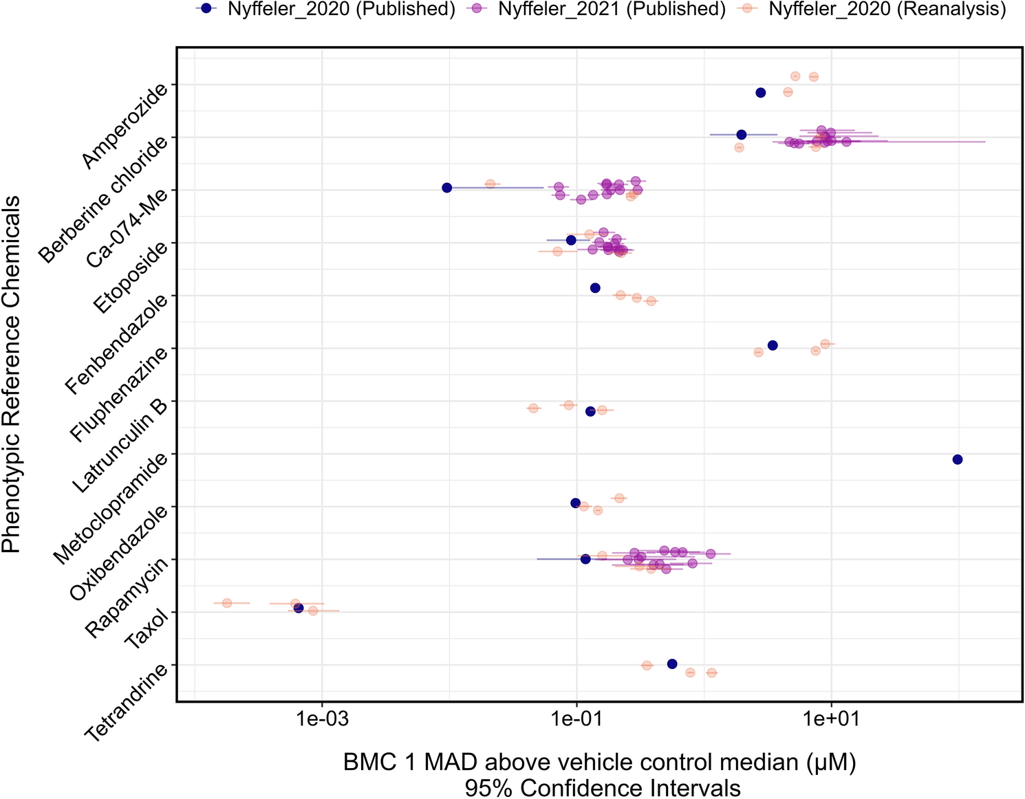
The tcplfit2 R package (Sheffield et al. 2022) was used to model concentration–response in the Mahalanobis distance in response to the phenotypic reference chemicals. As per the method used by Nyffeler et al. (2021), the benchmark response (BMR) for deriving the BMC was set as one MAD above the median Mahalanobis distance of the DMSO wells in the batch. The concentration–response of the Mahalanobis distance relative to the control compound (DMSO) was fitted to multiple models. The fit with the lowest Akaike Information Criterion (AIC) was selected as the winning model for each chemical. BMCs with a hitcall below 0.9 were excluded, as were BMCs that were above the highest tested concentration or without an upper or lower confidence limit.

Our pipeline was validated by processing publicly available well-level feature values from Nyffeler et al. (2020) (24-h exposures in U-2 OS cells in 51 384-well plates; URL: https://gaftp.epa.gov/COMPTOX/CCTE_Publication_Data/BCTD_Publication_Data/Nyffeler/) and comparing the BMCs produced using our pipeline against the published values in the 2020 and 2021 studies. The first 3 of the 51 published plates contained 14 phenotypic reference compounds only, and the remaining 48 plates included test chemicals with berberine chloride, Ca-074-Me, etoposide, and rapamycin as phenotypic positive controls.

To assess the impact of solvent control position on Mahalanobis distance calculations, the 96-well plate of U-2 OS cells treated only with 0.5% DMSO was normalized to the median of all wells or individual rows and columns. Each of the 12 columns and 8 rows were systematically designated as the solvent control in separate iterations, resulting in 20 total normalizations. Mahalanobis distances were recalculated for each set of normalized well-level feature values to evaluate the effect of control position across the plate.

Linear regression of Mahalanobis distance against cell count per well was performed using the lm() function from the R stats package. The strength of the association between these parameters was evaluated using the adjusted R-squared value.