Example: Maxwell Theory on a Spacelike Slice

We now give a succinct summary of Abelian YM theory on a 3-dimensional Riemannian manifold \((\Sigma ,\gamma )\)—thought of as a spacelike codimension-1 submanifold of M Lorentzian—as an exemplification of the theory outlined in Sect. 2. Details can be found in [85, 87].

For N a manifold, we denote \(\mathbb ^N \doteq C^\infty (N,\mathbb )\).

Let \(\mathcal = T^*\mathcal \ni (A,E)\), with \(A\in \mathcal \simeq \Omega ^1(\Sigma )\), \(E\in T^*_A\mathcal \simeq \Omega ^2(\Sigma )\), and \(\varvec= \mathbb E \wedge \mathbb A\), be the symplectic space of “magnetic potentials and electric fields” over \(\Sigma \). The (Abelian) gauge algebra is \(}= \mathbb ^\Sigma \); it acts on \(\mathcal \) as \(\rho (\xi )(A,E) = (d\xi ,0)\). Assume that the first de Rham cohomology of \(\Sigma \) is trivial, and denote n the normal to the boundary of \(\partial \Sigma \) and \(*\) the Hodge dual on \((\Sigma ,\gamma )\). Then, using the Hodge–Helmholtz decomposition, it is not hard to show that \(\mathcal _}\doteq \ \, \ d*A =0,\ i_n A |_ = 0\}\) is (the image of) a global section of \(\mathcal \rightarrow \mathcal /}\) and hence \(\mathcal _}\simeq \mathcal /}\).

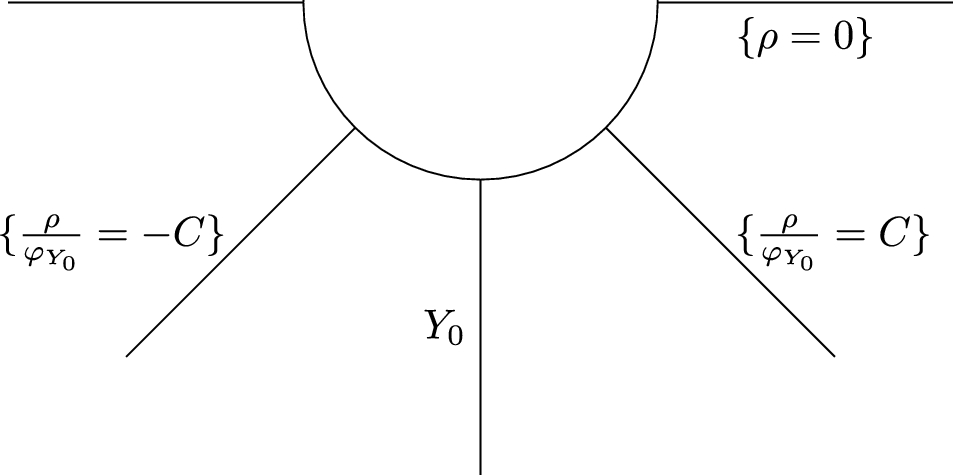
The momentum form \(}\) decomposes into the sum of a (Gauss) constraint form \(\langle }_\circ ,\xi \rangle = -\xi dE\), and a flux form \(\langle d},\xi \rangle = d(E\xi )\) which, once integrated on \(\Sigma \), gives the smeared electric flux through \(\partial \Sigma \). The constraint gauge group is \(}_\circ = \}\, \ \exists \chi \in \mathbb \text \xi |_=\chi \}\) (constant gauge transformations play a role because of Gauss’s law); the flux gauge group is \(\underline}}\simeq \mathbb ^/\mathbb \), where \(\mathbb \hookrightarrow \mathbb ^\) as constant functions, while flux space is found to be \(}\simeq \underline}}^* \simeq \textrm(\mathbb ,\mathbb ^)\).

The first- and second-stage reduced phase spaces are isomorphic (as symplectic or Poisson, resp.) manifolds to the following spaces:

$$\begin \underline}}\simeq T^*\mathcal _}\times T^*\underline}}\quad \text \quad }}}} \simeq T^*\mathcal _}\times \underline}}^* \end$$

Manifestly, \(\underline}}\) is a symplectic manifold, whereas \(}}}}\) is only Poisson. Since the flux space is \(}\simeq \underline}}^*\), the last formula states that all the superselection sectors are all isomorphic:

$$\begin \underline}}_ \simeq T^*\mathcal _}. \end$$

Physically \(T^*\mathcal _}\) encodes the radiative degrees of freedom (the “photons”) over \(\Sigma \), while \(}\simeq \underline}}^*\) encode the electric “Coulombic” degrees of freedom (i.e. the co-exact part of E, \(d\star \varphi \)) as parametrised by \(\iota _^*E|_\), the electric flux through \(\partial \Sigma \). This is possible because of the Gauss constraint \(}_\circ = dE\), which in the given decomposition is given by the equations \(\Delta \varphi = 0\) and \(i_nd\varphi |_ = \star _\iota _^*E\).

Note that, whereas in \(\underline}}\) the electric fluxes are conjugate to the gauge variant elements of \(\underline}}\)—sometimes called “edge modes” [28]—they have no symplectic partner in \(}}}}\). Indeed, in \(}}}}\), they are precisely the central coordinates in \(}}}}\) whose value labels the superselection sectors.

In the non-Abelian case, analogous results hold where \(T^*\underline}}\) is replaced by \(T^*\underline}}\), but the symplectomorphisms are only local [87, Section 6.5].

Notes on Definition 2.2 and Locality

The central notion used in the definition of a locally Hamiltonian gauge theory (Definition 2.2) is that of locality. Here, we briefly clarify this notion and refer to [87] for a detailed discussion (for a more general viewpoint see e.g. [11]).

1.

Let \(Y_\rightarrow \Sigma \), \(i=1,2\), be two fibre bundles, and \(\mathcal _=\Gamma (\Sigma ,Y_)\) the corresponding spaces of sections, denoted \(\varphi _\); then, a map \(f:\mathcal _1 \rightarrow \mathcal _2\) is said local iff \(\varphi _2(x) \doteq f(\varphi _1)(x)\) can be expressed as a function of x, \(\varphi _1(x)\), and a finite number of its derivatives (called the order of the map) also evaluated at x. A map of order 0 is said ultralocal.

2.

There exists a notion of “local forms” \(}\in \Omega _}^(\Sigma \times \mathcal ) \subset \Omega ^(\Sigma \times \mathcal )\) that generalises that of local maps and function(al)s discussed above [11]. We denote by (d, i, L) and \((\mathbb ,\mathbb ,\mathbb )\) the symbols of Cartan calculus on local forms \(\Omega _}^(\Sigma \times \mathcal )\). We will see that whereas Hamiltonian Yang–Mills theory on a spacelike \(\Sigma \) features an ultralocal symplectic density, Hamiltonian Yang–Mills theory on a null \(\Sigma \) does not.

3.

A (real) Lie algebra \(}\) is said local if its elements \(\xi \) are sections of a (real) vector bundle \(\Xi \rightarrow \Sigma \) and its Lie bracket \([\cdot ,\cdot ]: }\wedge }\rightarrow }\) is a local map.

4.

The action \(\rho :\mathcal \times }\rightarrow T\mathcal \) is said local iff it is a local map.

5.

Local \(\mathbb \)-linear maps \(}\rightarrow \Omega ^,0}(\Sigma \times \mathcal )\) can be identified with local forms \(\Omega _}^}(\Sigma \times \mathcal ,}^*_\textrm)\) valued in the local dual (defined in Remark 2.3), or with local forms in the triple complex \(\Omega _}^}(\Sigma \times \mathcal \times })\) which are linear in \(}\) [87, Defintion 2.12]. Throughout, we will deliberately merge these notions. With reference to the definition of a locally Hamiltonian gauge theory this means merging the momentum and co-momentum map viewpoints, and only talking about momentum forms and maps when referring to \(}\) and derived objects.

6.

The quantity \(d}(\xi ,\eta )\) is a Chevalley–Eilenberg cocycle of \(}\). It does not depend on the fields (\(\mathbb d}(\xi ,\eta )=0\)) [87, Sect. 3.5]. Its d-exactness is here imposed to match the Lagrangian origin of the locally Hamiltonian gauge theory, where equivariance up to a boundary cocycle is a consequence of Noether’s theorem and encodes the first-class nature of the gauge constraints [87, Appendix D].

Wilson Lines and Path-Ordered Exponentials

In this appendix, G denotes a Lie group which is either (i) Abelian, or (ii) compact and semisimple.

We begin with a statement about a 1-dimensional parallel transport problem for each of the k-components of the map \(Y:I\rightarrow \Omega ^k(S,})\); the lemma readily follows from the theory of ODEs in one variable:

Lemma C.1

(Parallel transport along \(\ell \)). Let \(Y,Z:I \rightarrow \Omega ^k(S,})\) and \(Z_0 = \Omega ^k(S,})\). Then, for all smooth \(A\in \mathcal \), Z and \(Z_0\), the boundary value problemFootnote 59

$$\begin \mathcal _\ell Y = Z\\ Y|_ = Z_0 \end\right. } \end$$

admits a unique smooth solution \(Y(u)=(Y(A,Z,Z_0))(u)\).

Next, we recall a standard result on the definition of Wilson lines (sometimes referred to as “holonomies” or “parallel transports”) of a gauge connection along the integral curves of \(\ell =\partial _u\):Footnote 60

Notation C.2

Let \(x\in S\). By definition \((L_\ell UU^)(x)\doteq i_\ell U_x^*\vartheta \), where \(U_x \doteq \textrm_x\circ U: I \rightarrow G\) and \(\vartheta \in \Omega ^(G,})\) is the right-invariant Maurer–Cartan form on G. This quantity is valued in \(C^\infty (S,}) = }^S\).

Lemma C.3

(Wilson lines along \(\ell \)). Let \(U\in C^\infty (I,G^S)\). Then, for all smooth \(A \in \mathcal \), the boundary value problem

$$\begin L_\ell ^ = - A_\ell \\ (u=+1) = 1 \end\right. } \end$$

admits a unique smooth solution \((u)=((A))(u)\), which we call the Wilson lines (of A along \(\ell \)), and denote

$$\begin ((A))(u) \equiv \overrightarrow} \int _u^ du' \ A_\ell (u'). \end$$

In the Abelian case one has the identity

$$\begin ((A))(u) = \exp \int _u^1 du' \, A_\ell (u') \quad \mathrm \end$$

Thanks to the smoothness and uniqueness of the Wilson lines \((A)\), one deduces:

Corollary C.4

(of Lemma C.3). The Wilson lines \((A) = \overrightarrow}\int A_\ell : I \rightarrow G^S\) can be interpreted as maps: \(\mathcal \rightarrow G^\Sigma \simeq C^\infty (I,G^S)\) which are bi-locally equivariant under the action of gauge transformations \(g \in G^\Sigma \),

$$\begin ((A^g))(u) = (g(u))^ ((A))(u) g^}. \end$$

In particular if \(A=g^ dg\),

$$\begin (( g^dg))(u) \equiv \overrightarrow} \int _u^ du' \ g^L_\ell g(u') = (g(u))^ g^}. \end$$

Proofs of Some Lemmas1.1 Proof of Lemma 4.5

Let \(\mathcal \subset \mathcal \) and \(\mathcal =\textrm(\mathcal ,\mathcal ^*_})\). From

$$\begin \textrm(\mathcal ,\mathcal ^*_}) \simeq \left( \mathcal /\mathcal \right) ^*_}, \quad \textrm(\mathcal ,\mathcal ) \simeq \left( \mathcal ^*_}/\mathcal \right) ^*_} \end$$

we obtain

Dualising the short exact sequence

$$\begin \mathcal \rightarrow \mathcal \rightarrow \mathcal /\mathcal \end$$

we conclude that \(\mathcal ^*_} \simeq \mathcal ^*_} / \left( \mathcal /\mathcal \right) ^*_}\). Hence, since both nuclear Freéchet vector spaces and their strong duals, as well as their closed subspaces,Footnote 61 are reflexive [62, Rmk. 6.5], one finds

1.2 The Two-Form of Definition 3.6 is Symplectic

According to Definition 2.2(ii), \(\varvec_\textsf\) of Definition 3.6 is a symplectic density iff \(\varvec_\textsf\) is \(\mathbb \)-closed and \(\omega _\textsf= \int _\Sigma \varvec_\textsf\) is (weakly) symplectic. The form \(\varvec_\textsf\) is obviously \(\mathbb \)-closed, and therefore so is \(\omega _\textsf\). Therefore, the crux is proving the (weak) non-degeneracy of \(\omega _\textsf\), i.e. \(\mathbb _}\omega _\textsf= 0\) iff \(\mathbb =0\).

For ease of notation, we henceforth drop the subscript \(\cdot _\textsf\), i.e. \(\varvec_\textsf\leadsto \varvec\), etc.

Using the identity of Eq. (2) for \(\mathbb F_\ell \), the form \(\varvec\) can be rewritten as

$$\begin \varvec= \Big ( \textrm(\mathbb E\wedge \mathbb A_\ell ) + \textrm( - \mathcal ^i \mathbb A_\ell \wedge \mathbb }_i) + \textrm( \mathcal _\ell \mathbb }^i \wedge \mathbb }_i) \Big )}_\Sigma . \end$$

Denoting

$$\begin \mathbb = \int X_E \frac + \hat^i \frac}^i} + X_\ell \frac, \end$$

one finds:

$$\begin \mathbb _\mathbb \varvec&= \Big ( \textrm(X_E \mathbb A_\ell ) - \textrm(\mathbb EX_\ell ) \\&\quad + \textrm( (\mathcal _\ell }^i - \mathcal ^i X_\ell ) \mathbb }_i) -\textrm( (\mathcal _\ell \mathbb }^i - \mathcal ^i\mathbb A_\ell ) }_i) \Big ) }_\Sigma . \end$$

Factoring out a total divergence (i.e. “integrating by parts”), one finds:

$$\begin \mathbb _\mathbb \varvec&= \Big ( - \textrm( X_\ell \mathbb E) + \textrm(X_E \mathbb A_\ell ) + \textrm( (\mathcal _\ell }^i ) \mathbb }_i) \nonumber \\&\quad + \textrm( (- \mathcal _\ell \mathbb }^i + \mathcal ^i\mathbb A_\ell ) }_i) \Big )}_\Sigma \end$$

(26a)

$$\begin&= \Big ( - \textrm( X_\ell \mathbb E) + \textrm( (X_E - \mathcal ^i }_i) \mathbb A_\ell ) + 2\textrm( (\mathcal _\ell }^i ) \mathbb }_i) \nonumber \\&\quad + D^i\textrm(}_i \mathbb A_\ell ) - \partial _u \textrm( }^i \mathbb }_i ) \Big )}_\Sigma \end$$

(26b)

$$\begin&\doteq (\mathbb _\mathbb \varvec)_\textrm + (\mathbb _\mathbb \varvec)_\textrm, \end$$

(26c)

where the “source” \((\textrm,1)\)-form \((\mathbb _\mathbb \varvec)_\textrm\) is defined by the first line of Eq. (26b), while the “boundary” \((\textrm,1)\)-form \((\mathbb _\mathbb \varvec)_\textrm\) is defined by the second line of the same equation.Footnote 62

We now use these formulas to prove that \(\omega \) is (weakly) non-degenerate, i.e. that if \(0 = \mathbb _\mathbb \omega = \int _\Sigma \mathbb _}\varvec\) then \(\mathbb =0\).

If \(0=\mathbb _\mathbb \omega \), then \(\mathbb _}\mathbb _\mathbb \omega =0\) for all \(\mathbb \) with \((Y_E, Y_\ell , }_i)\) of compact support in \(\mathring\), the open interior of \(\Sigma \). Using Takens’ theorem, we notice that for such \(\mathbb \)’s \(0=\mathbb _\mathbb \mathbb _\mathbb \omega = \int _\Sigma \mathbb _\mathbb (\mathbb _\mathbb \varvec)_\textrm\). From the fundamental lemma of the calculus of variations, it follows that \((\mathbb _\mathbb \varvec)_\textrm = 0\), that is:

$$\begin \mathbb _\mathbb \omega = 0 \implies (\mathbb _\mathbb \varvec)_\textrm = 0 \iff X_\ell = X_E - \mathcal ^i }_i = \mathcal _\ell }^i = 0, \end$$

where Eq. (26b) was used in the last step. Now recall that \(\mathbb _\mathbb \omega = \int _\Sigma (\mathbb _\mathbb \varvec)_\textrm + (\mathbb _\mathbb \varvec)_\textrm\). Leveraging the previous conditions, and using similar arguments, we also find that

$$\begin \mathbb _\mathbb \omega = 0 \implies 0 = \int _\Sigma \mathbb _\mathbb \varvec_} = \int _ \textbf(}^i \mathbb A_i) \iff }^i(u=\pm 1) = 0. \end$$

Combining this with the previous conditions on \(X_\ell \), \(X_E\) and \(\mathcal _\ell }^i\) as well as Lemma C.1, we conclude that \(\mathbb _\mathbb \omega =0\) implies \(X_\ell = X_E = }_i = 0\) i.e. \(\mathbb =0\).

Remark D.1

Staring from Eq. (26b), it is similarly possible to use Takens’s theorem (Footnote 62) and Lemma C.1 to show that \(\varvec\) is (weakly) non-degenerate, i.e. that \(\varvec^\flat \) is injective. However, in general, \(\varvec^\flat \) injective does not imply \(\omega ^\flat \) injective (in fact from the previous argument it is clear that the opposite is true, since \(\textrm(\varvec^\flat ) \subset \textrm(\omega ^\flat ) \subset \textrm(\varvec^\flat _\textrm)\)).

1.3 Proof of Lemma 3.9

Let \(f\in C^\infty (I,\mathbb )\) and define

$$\begin }(u) \doteq f(u) - ( f^0 - f^\textrm) - \fracf^\textrm. \end$$

Observe that

$$\begin }^0 = f^0 - 2 (f^0 - f^\textrm) = f^\textrm- (f^0 - f^\textrm) = }^\textrm, \end$$

whence, \(}^\textrm= 0= }^0 - }^\textrm\). In particular, \(}\) is \(C^\infty \) and periodic over I. Therefore, the partial Fourier series \(F_N[}]\),

$$\begin F_N[}](u)\doteq & \frac }}(0) + \sum _^N }}(k) \cos (\pi k u) + }}(k) \sin (\pi k u), \quad }}(k) + i }}(k) \\\doteq & \int _^1 }(u) e^, \end$$

converges to \(}\) uniformly. In particular,

$$\begin \frac }}(0) + \sum _^N (-1)^k }}(k) = F_N[}]^\textrm\rightarrow }^\textrm= }^0 = }}(0). \end$$

(27)

Moreover, note that the Fourier coefficients of f are related to those of \(}\) via

$$\begin a(k) + ib(k) \doteq \int _^1 f(u) e^ = }}(0) +2(f^0 - f^\textrm) & k=0,\\ }}(k) + i \left( }}(k)- \frac f^\textrm\right) & k\ge 1. \end\right. } \end$$

Consider now the partial series

$$\begin S_N[f](u) \doteq \sum _^N }(k)^*\psi _k(u) + c.c., \end$$

where

$$\begin 2}(k) \doteq 2\mathbb (\psi _k, f) = (f^0 - f^\textrm) + i f^\textrm& k=0\\ a(k) + i \left( 2 \pi k b(k) + 2(-1)^k f^\textrm\right) & k\ge 1 \end\right. } \end$$

(28)

Then, decomposing \(\psi _k=\psi ^R_k + i \psi ^I_k\), and \(} = }^R + i }^I\), into their real and imaginary parts,

$$\begin S_N[f](u)&= 2 \sum _^N\, \widetilde^R(k) \psi _k^R(u) + \,\widetilde^I(k) \psi _k^I(u) \\&= (f^0 - f^\textrm) + \frac f^\textrm+ \sum _^N }}(k) \psi _k^R(u) + 2\pi k }}(k) \psi ^I_k(u)\\&= (f^0 - f^\textrm) + \frac f^\textrm+ \sum _^N }}(k) ( (-1)^k + \cos (\pi k u) ) + }}(k) \sin (\pi k u)\\&= (f^0 - f^\textrm) + \frac f^\textrm+ F_N[}](u) - \frac }}(0) + \sum _^N (-1)^k }}(k) \end$$

where we used that for \(k\ge 1\), \(\bar(k)=a(k)\), as well as the expression for b(k) in terms of \(}(k)\). Finally, from the uniform convergence of the Fourier series \(F_N[}](u)\rightarrow }(u)\) and Eq. (27), we find

$$\begin S_N[f](u) \xrightarrow [N\rightarrow \infty ]} (f^0 - f^\textrm) + \frac f^\textrm+ }(u) = f(u). \end$$

1.4 Proof of Proposition 3.10

Generalising the result of Lemma 3.9 (Appendix D.3) to the case where \(f\in C^\infty (I)\) is replaced by \(}}\in \widehat}\simeq C^\infty (I,\Omega ^1(S))\), one finds

$$\begin S_N[}}_i(x)](u) \doteq \sum _^N \left( \, \widetilde}}}_i^* (k,x) \psi _k(u) + c.c. \right) \xrightarrow [N\rightarrow \infty ]} }}_i(u,x), \end$$

and thus

$$\begin }}&\doteq \int _S \int _^1 (L_\ell \mathbb }}_i(u,x)) \wedge \mathbb }}^i(u,x) du \ }_S \\&= 2i \int _S \mathbb ( \mathbb }}_i(x), \mathbb }}^i(x)) }_S\\&= 2i \int _S \lim _ \mathbb ( S_N[\mathbb }}_i(x)] , S_M[\mathbb }}^i(x)] ) }_S\\&= 2i \int _S \sum _^\infty \mathbb \, \widetilde}}}_i^*(k,x) \wedge \mathbb \, \widetilde}}}^i(k,x) }_S, \end$$

where in the third equality we used the fact that the convergence is uniform to pull out the limit from the integral over \(u\in I\) that is implicit in the definition of \(\mathbb \). The final expression of \(}}\) where the \(k=0\) term is singled out is straightforward.

1.5 Details of Calculation 5.18

We compute \(\omega (A^U,E^U)\). Recall Definition 3.6:

$$\begin \varvec(A,E) \doteq \textrm\big ( \mathbb F_\ell ^i \wedge \mathbb A_i + \mathbb E \wedge \mathbb A_\ell )}_\Sigma . \end$$

Thus, we compute:

$$\begin \varvec(A^U, E^U)&=\textrm\Big ( \mathbb (U^ F_^i U) \wedge \mathbb (U^ A_i U + U^\partial _i U) \nonumber \\&\quad + \mathbb (U^ E U) \wedge \mathbb (U^ A_\ell U + U^\partial _u\mathbb U\Big )}_\Sigma \nonumber \\&= \varvec(A,E) \nonumber \\&\quad + \textrm\Big ( [ F_^i,\mathbb U U^ ] \wedge \mathcal _i(\mathbb U U^) + [E, \mathbb U U^]\wedge \mathcal _\ell (\mathbb U U^)\Big )}_\Sigma \nonumber \\&\quad + \textrm\Big (\mathbb E \wedge \mathcal _\ell \mathbb U U^ - \mathbb F_^i \wedge \mathcal _i\mathbb U U^ \nonumber \\&\quad + [F_^i , \mathbb U U^] \wedge \mathbb A_i + [E,\mathbb U U^]\wedge \mathbb A_\ell \Big )}_\Sigma \end$$

(29)

We focus first on the second line of (29). Recalling that the Gauss constraint reads \(} = \mathcal _\ell E + \mathcal _i F_^i\), and using the identity

$$\begin[\mathbb U U^, \mathcal _\ell \mathbb U U^] = \tfrac \mathcal _\ell [\mathbb U U^,\mathbb U U^] = \mathcal _\ell \mathbb (\mathbb U U^), \end$$

we find:

$$\begin[2^\textrm]&= \textrm\Big ( F_^i [\mathbb U U^, \mathcal _i \mathbb U U^ ] + E [\mathbb U U^, \mathcal _\ell \mathbb U U^] \Big )}_\Sigma \\&= - \textrm\big ( } \mathbb (\mathbb U U^ ) \big )}_\Sigma \\&\quad + L_\ell \textrm\big ( E \mathbb (\mathbb U U^)\big )}_\Sigma + D_i \textrm\big ( F_\ell ^i \mathbb (\mathbb U U^) \big )}_\Sigma \end$$

Next, we focus on the third and fourth lines of (29). Using the following identity for the variation of the Gauss constraint,

$$\begin \textrm\big ( (\mathbb })\xi \big )&= \textrm\big ((\mathcal _\ell \mathbb E + \mathcal _i \mathbb F_^i + [\mathbb A_\ell , E] + [\mathbb A_i, F_^i])\xi \big ) \\&= \textrm\big ( - \mathbb E \ \mathcal _\ell \xi - \mathbb F_^i \ \mathcal _i\xi + [\mathbb A_\ell , E] \xi + [\mathbb A_i, F_^i] \xi \big ) \\ &\quad + L_\ell \textrm\big ( (\mathbb E) \xi \big ) + D_i\textrm\big ( (\mathbb F_^i) \xi \big ), \end$$

we find:

$$\begin[3^\textrm+4^\textrm]&= - \textrm(\mathbb } \wedge \mathbb U U^)}_\Sigma \\ &\quad + L_\ell \textrm\big ( \mathbb E \wedge \mathbb U U^\big )}_\Sigma + D_i\textrm\big ( \mathbb F_^i \wedge \mathbb U U^)}_\Sigma \\ \end$$

Summing the two contributions, we obtain:

$$\begin \varvec(A^U,E^U)&= \varvec(A,E) + \mathbb \textrm\big ( } \mathbb U U^ )}_\Sigma \\ &\quad + L_\ell \mathbb \textrm( E \mathbb U U^ )}_\Sigma + D_i \mathbb \textrm( F_\ell ^i \mathbb U U^)}_\Sigma , \end$$

and thus, integrating over \(\Sigma \simeq S \times I\), we conclude:

$$\begin \omega (A^U,E^U)&= \omega (A,E) + \mathbb \int _\Sigma \textbf\big ( } \mathbb U U^ ) \\ &\quad + \mathbb \int _}} \textbf\big ( E^}\mathbb U^}(U^})^ \big ) - \mathbb \int _}} \textbf\big ( E^}\mathbb U^}(U^})^ \big ). \end$$

Proof of Equation (13) on Abelian YM in Theorem 5.2

In this appendix we prove that

$$\begin (\underline}},\underline) \simeq (}^}_}},^}_}})\simeq _\textrm(_}},}}) \quad \mathrm , \end$$

where

$$\begin (}^}_}},^}_}})\doteq (\widehat}\times T^*}^S, }}+ \omega _S). \end$$

In other words, we prove that there exists a global symplectomorphism between \((\underline}},\underline) \simeq (}^}_}},^}_}})\).

The fact that \((}^}_}},^}_}})\) is locally symplectomorphic to \((_}},}})\) is straightforward and relies on the multi-valuedness of the \(\log : G_0^S \rightarrow }^S\). Moreover, we note that the local symplectomorphism \((\underline}},\underline) \simeq _\textrm(_}},}})\) was proved on general grounds in the main Sect. 5.

1.1 Preliminaries Notation E.1

If (the connected real Lie group) G is Abelian then it is the direct product of a torus and the real line. We write

$$\begin G\simeq \textrm(1)^t \times \mathbb ^ \quad \textrm\quad }\simeq (i\mathbb )^\times \mathbb ^. \end$$

Notation E.2

Recall that \(G\hookrightarrow G^\Sigma \) as the space of constant mapping functions. Then,

$$\begin G \cdot G^\Sigma _\textrm\equiv \}\, \ \exists k\in G\text g|_=k\}. \end$$

Lemma E.3

(Abelian winding number). Let \(g\in G \cdot G^\Sigma _\textrm\), then the following \(}\)-valued is valued in an integer lattice of \(}\hookrightarrow }^S\),

$$\begin w(g)\doteq \frac \int _^1 du' \ g^ L_\ell g(u') \in (i\mathbb )^t \times \. \end$$

Moreover, \(w(g_1g_2) = w(g_1) + w(g_2)\). We call w(g) the winding number of \(g^S\in G \cdot G^\Sigma _\textrm\).

Proof

Consider \(a\le b\) in I, and recall the identity (for \(g\in }\)):

$$\begin W(g; a,b) \doteq \exp \int _^b du'\, g^\partial _g = g^(a) g(b). \end$$

This formula can be read as the gauge-equivariance of the (Abelian) path-ordered exponential—i.e. at each \(x\in S\) this formula is the holonomy (a.k.a. Wilson line, see Appendix C), drawn at constant x, between \((x,u=a)\) and \((x,u=b)\) (see Appendix C). Then, if \(g\in } \cdot G^\Sigma _\textrm\), we have \(\exp 2\pi w(g) = W(g; -1,1) = 1\), and therefore \(w(g) \in i \mathbb ^ \times \\).

We conclude by observing that the additivity \(w(g_1g_2) = w(g_1) + w(g_2)\) follows immediately from the definition since

$$\begin (g_1g_2)^ L_\ell (g_1g_2) = g_2^g_1^ (L_\ell g_1 g_2 + g_1 L_\ell g_2) = g_1^ L_\ell g_1 + g_2^ L_\ell g_2. \end$$

\(\square \)

Recall that the space of on-shell fluxes is \(}\doteq \textrm(\iota _}^*h)\), the constraint gauge algebra is \(}_\circ \doteq \textrm(},}^\Sigma )\), and the constraint gauge group is \(}_\circ \doteq \langle \exp }_\circ \rangle \). Now, if G is Abelian, Proposition 5.8(2) tells us that

$$\begin }_\circ \simeq }^\Sigma _\textrm+ }, \end$$

and

$$\begin }_\circ \doteq \langle \exp }_\circ \rangle \simeq (G\cdot G^\Sigma _\textrm)_0 = G\cdot G^\Sigma _,0}. \end$$

The next proposition provides a more explicit characterisation of \(}_\circ \):

Proposition E.4

(Abelian constraint gauge group \(}_\circ \)). The Abelian constraint gauge group \(}_\circ \doteq \langle \textrm}_\circ \rangle \) is isomorphic to

$$\begin }_\circ \simeq G\cdot G^\Sigma _,0} = \left\\, \ w(g) \doteq \tfrac (g^\partial _u g)^ = 0 \right\} . \end$$

Proof

We prove the statement by showing the two inclusions.

Lemma E.3 states that w(g) is valued in an integer lattice \((i\mathbb )^\times \\subset }\hookrightarrow }^S\). But then, since \(w(g)\in }^S\) is continuous over S, w(g) is constant on S. Additionally, \(w:G \cdot G^\Sigma _\textrm\rightarrow }\) is a constant function over the connected components of \(G \cdot G^\Sigma _\textrm\)—and in particular it vanishes on the identity component. Therefore:

$$\begin G\cdot G^\Sigma _,0} \subset \\, \ w(g) = 0 \}. \end$$

Next, let \(g\in G\cdot G^\Sigma _\textrm\)—so that \(g^}=g^}\equiv k\in G\)—and assume \(w(g)=0\). For all \(t\in [0,1]\), define

$$\begin g_t \doteq k \exp t \int _^u du' \, g^L_\ell g(u'). \end$$

Then, \(g_= g^}\) and \(g_ = k (g^)^}g = g\). Moreover, since \(w(g) = 0\), we have that \(g_t^}= k \exp (2\pi t w(g) ) = k\). Therefore for all \(t\in [0,1]\), \(g_t^}= g_t^}= k\in G\) and hence \(g_t \in G\cdot G^\Sigma _\textrm\). We thus conclude that \(g_t\) is an homotopy in \(G\cdot G^\Sigma _\textrm\) between g and a constant \(k\in G\). Since G is by hypothesis connected, g is not only homotopic within \(G\cdot G^\Sigma _\textrm\) to k but also to the identity \(1\in G\cdot G^\Sigma _\textrm\). Thus,

$$\begin G\cdot G^\Sigma _,0} \supseteq \\, \ w(g) = 0 \}. \end$$

\(\square \)

Remark E.5

(Group homomorphism). Recall Notation E.1. If \(t=0\) then it is easy to see that any \(g\in G\cdot G^\Sigma _\textrm\) is homotopic to the identity, and thus \(}_\circ =G\cdot G^\Sigma _\textrm\). On the other hand, if \(G=\textrm(1)\) and \(n\in \mathbb \), then the only element \(g^(u,x) = -\exp ( \pi n i u)\in G\cdot G^\Sigma _\textrm\) that is also in the identity component \(}_\circ = G\cdot G^\Sigma _,0}= \exp }_\circ \) is the identity itself, i.e. \(g^\).Footnote 63 The quantity w(g) is a topological invariant classifying the connected components of \(G\cdot G^\Sigma _\textrm\); in particular \(w(g^) = i n\). Moreover, \(w(g_1g_2)=w(g_1)+w(g_2)\). Indeed, if \(S =S^\) and \(n\ne 2\), the winding number w(g) provides a group homomorphism between \(G\cdot G^\Sigma _\textrm\) and the group of components of \(G\cdot G^\Sigma _\textrm\simeq G^ \simeq \mathbb ^t\).

1.2 Gauge Fixing

We now turn our attention to the action of the constraint gauge group on the constraint surface \(}\subset \mathcal \). Since \(}_\circ \simeq }^\Sigma _\textrm+ }\) “differs” from \(}^\Sigma _\textrm\) only by the (\(}\)-global) isotropy \(\textrm(\rho ) = }\hookrightarrow }\), one has

$$\begin \underline}}\doteq }/ }_\circ = }/ G^\Sigma _,0}. \end$$

Recall Proposition 4.2 which states that

$$\begin }\simeq \mathcal \times (}^S)^*. \end$$

Lemma E.6

The action of \(G^\Sigma _,0}\) on \(}\) induces the following action of \(G^\Sigma _,0}\) on \(\mathcal \times }^S)^*}\):

$$\begin G^\Sigma _,0} \circlearrowright \mathcal \times }^S)^*}, \quad (g_\circ , A, }}) \mapsto (A^, }}). \end$$

This action defines the principal \(G^\Sigma _,0}\)-bundle

$$\begin \underline_\circ :\mathcal \times }^S)^*} \rightarrow (\mathcal \times }^S)^*})/G^\Sigma _,0}, \end$$

with \((\mathcal \times }^S)^*})/G^\Sigma _,0} = (\mathcal \times }^S)^*})/}_\circ \simeq \underline}}\). Diagrammatically:

Proof

The only step of the proof that is not obvious and requires some care is proving that the action of \(G^\Sigma _,0}\) is free on \(\mathcal \) and therefore on \(\mathcal \times }^S)^*}\). This follows from \(\textrm(\rho ) = }\hookrightarrow }^\Sigma \) and \(}\cap }^\Sigma _\textrm= \\). \(\square \)

Now, since \(}\simeq \mathcal \times (}^S)^*\) is a principal \(G^\Sigma _,0}\)-bundle and \(\underline}}\doteq }/}_\circ \simeq }/G^\Sigma _,0}\), the question of reduction can be directly addressed if we can find a (global) gauge fixing of the action of \(G^\Sigma _,0}\) on \(}\), i.e. a (global) section of the principal \(G^\Sigma _,0}\)-bundle \((\mathcal \times (}^S)^*, }_\circ )\). We proceed in two steps: first we introduce a trivialisation of this principal bundle, and then leverage it to construct a global section.

Lemma E.7

Viewing \( G^\Sigma _,0} \subset G^\Sigma \simeq C^\infty (I,G^S)\), let

$$\begin & :\mathcal \rightarrow }^\Sigma \simeq C^\infty (I,}^S), \quad \\ & A \mapsto ((A))(u)\doteq - \int _^u du' \,A_\ell (u') + \tfrac (u+1) (A_\ell )^. \end$$

Then, the following map is a principal \(G^\Sigma _,0}\)-bundle trivialisation:

$$\begin \begin \underline_\circ : &\mathcal \times (}^S)^* \rightarrow }^}_}}\times G^\Sigma _,0} \equiv \widehat}\times T^*}^S \times G^\Sigma _,0}\\ \\ & \,\; \begin A\\ }} \end \;\mapsto \begin }}(A)\\ \\ }}(E_}) \\ (A) \end \doteq \begin \hat + D(A) - \tfrac (u-1) D(A_\ell )^\\ (A_\ell )^\\ }}\\ \exp (A) \end \end \end$$

where \(}}}\in T_^*}^S\simeq (}^S)^*\) (cf. Remark 4.1). Diagrammatically:

where \(\pi _\) denotes the projection on the first two factors, and we have \(\underline_\circ = \pi _ \circ \underline_\circ \).

Proof

Proving the lemma requires showing that (1) \(\underline_\circ \) is invertible, and (2) it maps right-translations of the \(G^\Sigma _,0}\)-factor in \(\widehat}\times T^*}^S\times ,0}}\) onto the action of \(,0}}\) on \(\mathcal \times }^S)^*}\). Throughout the proof, it is useful to keep in mind that \(\lambda (A)\) is constant in u.

To prove (1), it is enough to show that the following map is indeed both a left and a right inverse of \(}_\circ \):

$$\begin }_\circ ^ :\widehat}\times T^*}^S \times ,0}}&\rightarrow \mathcal \times }^S)^*}\nonumber \\ (}},\lambda ,}},)&\mapsto \begin A \\ E_}\end \nonumber \\&= \begin }}+ \tfrac(u-1)D\lambda + \tfrac\lambda du - d^\\ }}\end. \end$$

(30)

Proving the left-inverse property is straightforward once one notices that the first component \(}}(A)}\) of \(\underline_\circ (A,}})\) satisfies

$$\begin }}(A)} + \tfrac(u-1)D\lambda (A) + \tfrac\lambda (A) du = A + (A)^ d(A). \end$$

We leave the details to the reader.

Proving the right-inverse property is instead subtler. For this we need some preliminary results. Denote the first component of \(}_\circ ^(}},\lambda ,}},U_\circ )\) by

$$\begin A'=A'(}},\lambda ,}},) \doteq }}+ \tfrac(u-1)D\lambda + \tfrac\lambda du - d^. \end$$

Then,

$$\begin A'_\ell = \tfrac \lambda - L_\ell ^. \end$$

From these, recalling that \(\lambda \) is constant in u, we compute:

$$\begin \lambda (A') \doteq ( A'_\ell )^ = \lambda - (L_\ell ^)^ = \lambda \end$$

where we used the fact that \(U_\circ \in G^\Sigma _,0}\) and therefore \( w(U_\circ )= \frac(U_\circ ^L_\ell U_\circ )^=0\) (Proposition E.4). Similarly, we find

$$\begin ((A'))(u)\doteq - \int _^u du'\, A'_\ell + \tfrac(u+1) (A'_\ell )^ = - \int _^u du'\, U_\circ ^L_\ell U_\circ (u'), \end$$

and thus (see also Appendix C)

$$\begin (A') \doteq \exp (A') = (^})^= . \end$$

Now, with these two formulas, it is easy to see that \(}_\circ ^\) is indeed a right inverse of \(\underline_\circ \) as well. This concludes the proof of (1).

Finally, to prove (2) we appeal to (1) which tells us that it is enough to prove that \(U_\circ \mapsto g_\circ U_\circ \) maps \(A' \mapsto A' + g_\circ ^d g_\circ \), a fact that is obvious when looking at the explicit form of \(}_\circ ^\). \(\square \)

Now that we have an explicit, global, trivialisation \(\underline_\circ \) of the principal \(G^\Sigma _,0}\)-bundle \(\underline_\circ :\mathcal \times (}^S)^*\rightarrow \widehat}\times T^*}^S\), it is immediate to produce one of its (global) sections, \(\underline_\circ \):

Corollary E.8

The map \(\underline_\circ : }^}_}}\rightarrow \mathcal \times (}^S)^*\) defined as

$$\begin \underline_\circ \doteq \underline^_\circ ( \cdot ,\cdot ,\cdot ,1), \end$$

where \(1 \in G^\Sigma _,0}\) (cf. Equation (30)), is a section of \(\mathcal \times (}^S)^* \xrightarrow _\