2.1 The Entanglement Entropy of a Quasi-Free Fermionic State

Given a Hilbert space \((\mathscr _m, \langle .|. \rangle _m\)) (the “one-particle Hilbert space”), we let \((}, \) \(\langle .|. \rangle _})\) be the corresponding fermionic Fock space, i.e.,

$$\begin } = \bigoplus _^\infty \;\underbrace_m \wedge \cdots \wedge \mathscr _m}_} \end$$

(where \(\wedge \) denotes the totally anti-symmetrized tensor product). We define the creation operator \(\Psi ^\dagger \) by

$$\begin \Psi ^\dagger \,:\, \mathscr _m \rightarrow }(}) \,,\qquad \Psi ^\dagger (\psi ) \big ( \psi _1 \wedge \cdots \wedge \psi _p \big ):= \psi \wedge \psi _1 \wedge \cdots \wedge \psi _p \,. \end$$

Its adjoint is the annihilation operator denoted by \(\Psi (}):= (\Psi ^\dagger (\psi ))^*\). These operators satisfy the canonical anti-commutation relations

$$\begin \big \}), \Psi ^\dagger (\phi ) \big \} = ( \psi | \phi ) \qquad \text \qquad \big \}), \Psi (}) \big \} = 0 = \big \ \,. \end$$

Next, we let W be a statistical operator on \(}\), i.e., a positive semi-definite linear operator of trace one,

$$\begin W \,:\, }\rightarrow }\,,\qquad W \ge 0 \quad \text \quad \,}}_}(W)=1 \,. \end$$

Given an observable A (i.e., a symmetric operator on \(}\)), the expectation value of the measurement is given by

$$\begin \langle A \rangle := \,}}_}\big ( A W) \,. \end$$

The corresponding quantum state \(\Omega \) is the linear functional which to every observable associates the expectation value, i.e.,

$$\begin \Omega \,:\, A \mapsto \,}}_}\big ( A W) \,. \end$$

In this work, we restrict our attention to the subclass of so-called quasi-free quantum states, fully determined by their two-point functions

$$\begin \Omega _2(}, \phi ):= \Omega \big (\Psi ^\dagger (\phi ) \, \Psi (}) \big ) \,, \qquad \text \text \psi , \phi \in }_m \,. \end$$

Definition 2.1

The reduced one-particle density operator D is the positive linear operator on the Hilbert space  defined by

$$\begin \Omega _2(}, \phi ) = \langle \psi \,|\, D \phi \rangle _m \,, \qquad \text \psi , \phi \in }_m \,. \end$$

The von Neumann entropy \(S(\Omega )\) of the quasi-free fermionic state \(\Omega \) can be expressed in terms of the reduced one-particle density operator by

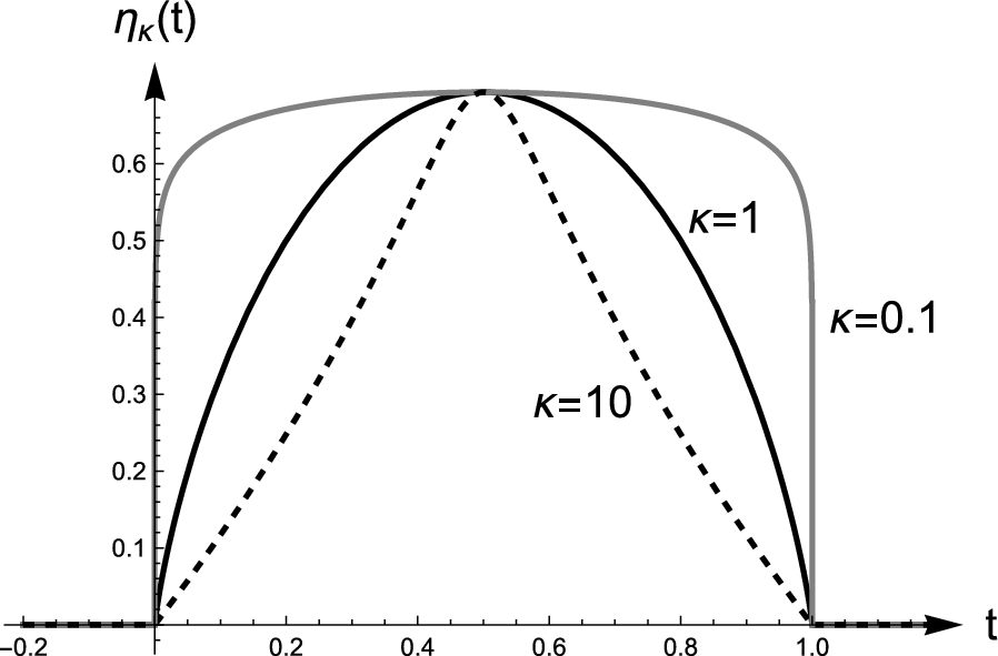
$$\begin S(\Omega ) = \,}}\eta _1(D) \,, \end$$

(2.1)

where \(\eta _\kappa \) is the function from (1.2) (for a plot, see Fig. 1). This formula appears commonly in the literature (see, for example, [28, Equation 6.3], [7, 22, 26] and [20, eq. (34)]). A detailed derivation is found in [11, Appendix A]. Similar to (2.1) also other entropies can be expressed in terms of the reduced one-particle density operator. In particular, the Rényi entropy can be written as \(S_\kappa (\Omega ) = \,}}\eta _\kappa (D)\) This formula is also derived in [11, Appendix A].

For the entanglement entropy, we need to assume that the Hilbert space \(\mathscr _m\) is formed of wave functions in spacetime. Restricting them to a Cauchy surface, we obtain functions defined on three-dimensional space  (which could be \(\mathbb ^3\) or, more generally, a three-dimensional manifold). Given a spatial subregion , we define the (Rényi) entanglement entropy by

$$\begin S_\kappa (D, \Lambda ) := \,}}\big ( \eta _\kappa \big ( \chi _ \,D\, \chi _ \big ) -\chi _ \,\eta _\kappa (D)\,\chi _ \big ) \,. \end$$

(2.2)

More details in the case \(\kappa =1\) can be found in [24, Section 3].

2.2 The Dirac Equation in Globally Hyperbolic Spacetimes

Since we are ultimately interested in Schwarzschild space time, the abstract setting for the Dirac equation is given as follows (for more details see, for example, [12]). Our starting point is a four dimensional, smooth, globally hyperbolic Lorentzian spin manifold , with metric g of signature \((+,-, -, -)\). We denote the corresponding spinor bundle by . Its fibers  are endowed with an inner product  of signature (2, 2), referred to as the spin inner product. Moreover, the mapping

where the \(\gamma ^j\) are the Dirac matrices defined via the anti-commutation relations

provides the structure of a Clifford multiplication.

Smooth sections in the spinor bundle are denoted by . Likewise, are the smooth sections with compact support. We also refer to sections in the spinor bundle as wave functions. The Dirac operator \(}\) takes the form

where \(\nabla \) denotes the connections on the tangent bundle and the spinor bundle. Then the Dirac equation with parameter m (in the physical context corresponding to the particle mass) reads

$$\begin (}- m) \,\psi = 0 \,. \end$$

(2.3)

Due to global hyperbolicity, our spacetime admits a foliation by Cauchy surfaces . Smooth initial data on any such Cauchy surface yield a unique global solution of the Dirac equation. Our main focus lies on smooth solutions with spatially compact support, denoted by . The solutions in this class are endowed with the scalar product

(2.4)

where  is a Cauchy surface  with future-directed normal \(\nu \) and  denotes the measure on  induced by the metric g (compared to the conventions in [12], we here preferred to leave out a factor of \(2 \pi \)). This scalar product is independent of the choice of  (for details see [12, Section 2]). Finally, we define the Hilbert space \((\mathscr _m, (.|.)_m)\) by completion,

2.3 The Dirac Propagator in the Schwarzschild Geometry2.3.1 The Integral Representation of the Propagator

We recall the form of the Dirac equation in the Schwarzschild geometry and its separation, closely following the presentation in [8] and [14]. Given a parameter \(M>0\) (the black hole mass), the exterior Schwarzschild metric reads

$$\begin \textrms^2 = g_\,\textrmx^j \,\textrmx^k = \frac \, \textrmt^2 - \frac\,\textrmr^2 - r^2\, \textrm \vartheta ^2 - r^2\, \sin ^2 \vartheta \, \textrm\varphi ^2\,, \end$$

where

$$\begin \Delta (r):= r^2 - 2M r \,. \end$$

Here the coordinates \((t, r, \vartheta , \varphi )\) take values in the intervals

$$\begin -\infty<t<\infty ,\qquad r_1<r<\infty ,\qquad 0<\vartheta<\pi ,\qquad 0<\varphi <2\pi \,, \end$$

where \(r_1:=2M\) is the event horizon. It is most convenient to transform the radial coordinate to the so called Regge–Wheeler coordinate \(u \in \mathbb \) defined by

$$\begin u(r) = r + 2M \log (r-2M)\,, \qquad \text \qquad \fracu}r} = \frac\,. \end$$

(2.5)

In this coordinate, the event horizon is located at \(u \rightarrow - \infty \), whereas \(u\rightarrow \infty \) corresponds to spatial infinity, i.e., \(r \rightarrow \infty \).

In this geometry, the Dirac operator takes the form (see also [14, Section 2.2]):

$$\begin }&= \begin 0 & 0 & \alpha _+ & \beta _+ \\ 0 & 0 & \beta _- & \alpha _- \\ \alpha _- & -\beta _+ & 0 & 0 \\ -\beta _- & \alpha _+ & 0 & 0 \end \qquad \text \\ \beta _\pm&= \frac \left( \frac + \frac \right) \pm \frac \,\frac \qquad \text \\ \alpha _\pm&= -\frac} \,\frac \pm \frac} \left( i \frac \,+\, i \,\frac \,+\, \frac \right) . \end$$

Then the Dirac equation can be separated with the ansatz

$$\begin \psi ^(t,u,\varphi ,\vartheta ) = e^\,\frac \sqrt}\, \begin X_-^(t,u)Y^_-(\vartheta )\\ X_+^(t,u)Y^_+(\vartheta )\\ X_+^(t,u)Y^_-(\vartheta )\\ X_-^(t,u)Y^_+(\vartheta ) \end \end$$

with \(k \in \mathbb +1/2\), \(n \in \mathbb \) and \(\omega \in \mathbb \). The angular functions \(Y^_\pm \) can be expressed in terms of spin-weighted spherical harmonics and form an orthonormal basis of \(L^2\big (\big ((-1,1),\,\textrm\vartheta \cos \vartheta \big ), \mathbb ^2\big )\) (see [14, Section 2.4] with additional reference to [15]). The radial functions \(X^_\pm \) satisfy a system of partial differential equations

$$\begin \begin \sqrt\, }_+ & imr-\lambda \\ -imr-\lambda & \sqrt\, }_- \end \begin X_+^ \\ X_-^ \end = 0\,, \end$$

(2.6)

where m denotes the particle mass and

$$\begin }_\pm = \frac \mp \frac\,\frac \,, \end$$

for details see [8, Section 2]. Moreover, employing the ansatz

$$\begin X^_\pm (t,u)= e^ \,X^_\pm (u) \,, \end$$

equation (2.6) goes over to a system of ordinary differential equations, which admits two two-component fundamental solutions labeled by \(a=1,2\). We denote the resulting Dirac solution by \(X^_a=(X^_, X^_)\). In the case \(|\omega |<m\), these solutions behave exponentially near infinity. We always choose the fundamental solution for

$$\begin a=1\text decays\text \end$$

(2.7)

For more details on the choice of the fundamental solutions, see Sect. 2.3.4.

In what follows, we will often use the following notation for two-component functions

$$\begin A:=\begin A_+ \\ A_- \end\,. \end$$

The norm in \(\mathbb ^2\) will be denoted by \(| .\, |\), the canonical inner product on \(L^2(\mathbb ,\mathbb ^2)\) by \(\langle .|.\rangle \) and the corresponding norm by \(\Vert .\Vert \).

As implied by [8, Theorem 3.6], one can then find the following formula for the mode-wise propagator:

Theorem 2.2

Given initial radial data \(X_0 \in C^\infty _0(\mathbb , \mathbb ^2)\) at time \(t=0\), the corresponding solution \(X \in C^\infty (\mathbb ^2,\mathbb ^2)\) of the radial Dirac equation (2.6) can be written as

$$\begin X(t, u) = \frac \int _^\infty \textrm\omega \,e^ \sum _^ t_^ \,X_a^ (u) \,\langle X_b^ | X_0 \rangle \,, \end$$

(2.8)

for any \(t,u \in \mathbb \). The \(X_a^ (x)\) are the fundamental solutions mentioned before. Here the coefficients \(t_^\) satisfy the relations

$$\begin \overline_} = t^_ \end$$

and

$$\begin \left\ t^_ = \delta _ \,\delta _ & \qquad \text |\omega | \le m \\ \displaystyle t^_ = t_=\frac\,,\quad \big |t^_ \big | \le \frac & \qquad \text |\omega | > m\,. \end \right. \end$$

(2.9)

We note for clarity that, in view of (2.9) and (2.7), in the case \(|\omega |<m\) only the exponentially decaying wave function enters the integral representation. This has the effect that, asymptotically near infinity, only the spectrum for \(|\omega | \ge m\) is visible, in agreement with the mass gap in Minkowski space.

2.3.2 Hamiltonian Formulation

The Dirac equation (2.3) can be written in the Hamiltonian form

$$\begin i \partial _t \psi = H \psi \,, \end$$

(2.10)

where the Hamiltonian H is a spatial operator acting on the spinors. Choosing the Cauchy surface  as the surface of constant Schwarzschild time and the domain \(\mathscr (H)\) as the smooth and compactly supported spinorial wave functions on , the Hamiltonian is symmetric with respect to the scalar product (2.4), i.e.,

$$\begin (H \psi \,|\, \phi )_m = (\psi \,|\, H \phi )_m \qquad \text \psi , \phi \in \mathscr (H) \end$$

(for more details on this point in general stationary spacetimes, see [9, Section 4.6]). The Hamiltonian is essentially self-adjoint (see [13] for details in a more general context). Denoting the unique self-adjoint extension again by H, the Cauchy problem can be solved with the spectral calculus by

$$\begin \psi (t) = e^\, \psi _0 \,. \end$$

(2.11)

This is the abstract counterpart of the integral representation of Theorem 2.2. In simple terms, the solution (2.8) can be understood as giving an integral representation for the operator \(e^\) restricted to an angular mode. Noting that \(\omega \) is the spectral parameter, the integral in (2.8) can be understood as a spectral decomposition in terms of the spectral measure (in particular, the spectrum of the Hamiltonian is the whole real axis). In order to make these connections more precise, we first note that also the radial Dirac equation after separation of variables (2.6) can be written in the Hamiltonian form

$$\begin&i \frac X^ (t,u)= \big (H_ X^|_t\big )(u) \\ \Longleftrightarrow \qquad&(}- m)\,e^\,\frac \sqrt}\, \begin X^_-(t,u)Y^_-(\vartheta )\\ X^_+(t,u)Y^_+(\vartheta )\\ X^_+(t,u)Y^_-(\vartheta )\\ X^_-(t,u)Y^_+(\vartheta ) \end = 0 \;, \end$$

where the Hamiltonian \(H_\) now is an essentially self-adjoint operator on  \(L^2(\mathbb ,\mathbb ^2)\) with dense domain \(\mathscr (H_) = C^\infty _0(\mathbb ,\mathbb ^2 )\). This makes it possible to write the solution of the Cauchy problem as

$$\begin X (t,u) = \big (e^} \,X_0 \big )(u) \qquad \text u \in \mathbb \,. \end$$

Here, the initial data can be an arbitrary vector-valued function in the Hilbert space, i.e., \(X_0 \in L^2(\mathbb ,\mathbb ^2)\). If we specialize to smooth initial data with compact support, i.e., \(X_0 \in C^\infty _0(\mathbb ,\mathbb ^2)\), then the time evolution operator can be written with the help of Theorem 2.2 as

$$\begin \big (e^} X_0 \big )(u)&= \frac \int _^\infty \textrm\omega \,e^ \sum _^ t_^&\,X_a^ (u) \,\langle X_b^ | X_0 \rangle \\&\qquad \text X_0 \in C^\infty _0(\mathbb ,\mathbb ^2) \end$$

We point out that this formula does not immediately extend to general \(X_0 \in L^2(\mathbb ,\mathbb ^2)\); we will come back to this technical issue a few times in this work.

2.3.3 Connection to the Full Propagator

We now explain how the solution of the Cauchy problem as given abstractly in (2.11) can be decomposed into angular modes. Our considerations explain why we may restrict attention to one angular mode instead of the full propagator and why we can use the ordinary \(L^2\)-scalar product instead of \((.|.)_m\). We introduce the function

$$\begin S:=\Delta (r)^ \sqrt \,. \end$$

Moreover, for each fixed \(k \in \mathbb +1/2\) and \(n\in \mathbb \) we denote by \((\mathscr _m^0)_\) the completion of the vector space

$$\begin V_:= \left\\,e^ \,\begin X^_-(u)Y^_-(\vartheta )\\ X^_+(u)Y^_+(\vartheta )\\ X^_+(u)Y^_-(\vartheta )\\ X^_-(u)Y^_+(\vartheta ) \end \, \bigg |\, X=(X_+,X_-) \in L^2(\mathbb ,\mathbb ^2)\right\} \,, \end$$

with respect to the scalar product \((.|.)_m\) introduced in (2.4), i.e.,

$$\begin (\mathscr _m^0)_:= \overline}^ \,. \end$$

This space can be thought of as the mode-wise solution space of the Dirac equation at time \(t=0\). Note that the entire Hilbert space of solutions at time \(t=0\), namely

$$\begin \mathscr _m|_ =: \mathscr _m^0 \end$$

has the orthogonal decomposition

$$\begin \mathscr _m^0 = \bigoplus _} (\mathscr _m^0)_ \,. \end$$

(2.12)

(again with respect to \((.|.)_m\)), where \(((k_i,n_i))_}\) is an enumeration of \((\mathbb +1/2)\times \mathbb \). Furthermore, each space \((\mathscr _m^0)_\) can be connected with \(L^2(\mathbb ,\mathbb ^2)\) using the mapping

$$\begin }: \big ((\mathscr ^0_m)_ \,,\, (.|.) \big )&\rightarrow L^2(\mathbb , \mathbb ^2)\,, \end$$

which for any \((\psi _1, \cdots , \psi _4) \in (\mathscr ^0_m)_\) is given by

$$\begin&\big ( }(\psi _1, \cdots , \psi _4)\big )_1 \\&\quad = \int _^1 \textrm \vartheta \,\cos \vartheta \int _0^ \textrm\varphi \,\Big \langle \big ( \psi _2(u, \vartheta , \varphi ) \,, \, \psi _3(u, \vartheta , \varphi ) \big ) \,\Big |\, e^ \,\big ( Y^_+(\vartheta )\,, \, Y^_-(\vartheta ) \big ) \Big \rangle _^2} \,,\\&\big ( }(\psi _1, \cdots , \psi _4)\big )_2 \\&\quad = \int _^1 \textrm \vartheta \,\cos \vartheta \int _0^ \textrm\varphi \, \Big \langle \big ( \psi _4(u, \vartheta , \varphi ) \,, \, \psi _1(u, \vartheta , \varphi ) \big ) \,\Big |\, e^ \,\big ( Y^_+(\vartheta )\,, \, Y^_-(\vartheta ) \big ) \Big \rangle _^2} \,. \end$$

It has the inverse

$$\begin }^: L^2(\mathbb , \mathbb ^2)&\rightarrow \big ((\mathscr _m^0)_\,,\, (.|.)_m\big )\,, \\ (X_+,X_-)&\mapsto S^e^ \begin X_-(u)Y^_-(\vartheta )\\ X_+(u)Y^_+(\vartheta )\\ X_+(u)Y^_-(\vartheta )\\ X_-(u)Y^_+(\vartheta ) \end\,. \end$$

Then a direct computation shows the scalar products transform as

$$\begin \langle } \psi \, |\, } \phi \rangle _ =(\psi \,| \, \phi )_m \qquad \text \phi ,\psi \in (\mathscr _m^0)_\,. \end$$

This implies that \(}\) is unitary and we can identify the two spaces.

Now recall that the Dirac equation can be separated by solutions of the form

$$\begin }= S^ e^ \begin X_-(t,u)Y^_-(\vartheta )\\ X_+(t,u)Y^_+(\vartheta )\\ X_+(t,u)Y^_-(\vartheta )\\ X_-(t,u)Y^_+(\vartheta ) \end \,, \end$$

and can then be described mode-wise by the Hamiltonian \(H_\) on the space \(L^2\) \((\mathbb , \mathbb ^2)\). Therefore, denoting

$$\begin }_:=}^H_ } \,,\end$$

the diagonal block operator (with respect to the decomposition (2.12))

$$\begin }:=\text \big (}_\,,\, }_\,, \, \dots \,\big )\,, \end$$

defines an essentially self-adjoint Hamiltonian for the original Dirac equation on the space \(\mathscr _m^0\).

Moreover, any function of \(}\) is of the same diagonal block operator form. The same holds for any multiplication operator \(}_}}}\), where \(}\) is a spherically symmetric set

$$\begin }:= U \times S^2 \subseteq \mathbb \times S^2 \,.\end$$

In particular, such an operator has the block operator representation

$$\begin }_}}} = \text \big ( }_}}} \,,\, }_}}} \,,\, \dots \big ) \,. \end$$

We therefore conclude that when computing traces of operators of the form

$$\begin \chi _}}f(}) \chi _}}\qquad \text \qquad f(\chi _}} }\chi _}}) \,, \end$$

(for some suitable function f), we may consider each angular mode separately and then sum over the occupied states (and similarly for Schatten norms of such operators).

Moreover, we point out that instead of \((\mathscr _m^0)_\) we can work with the corresponding objects in \(L^2(\mathbb ,\mathbb ^2)\), as the spaces are unitarily equivalent. Note that then the multiplication operator \(}_}}}\) goes over to \(}_}\), i.e.,

$$\begin }^ }_}}}} = }_} \,.\end$$

In particular, this leads to

$$\begin \,}}\Big ( \chi _}}f(}) \chi _}} \Big ) = \, \sum _ \, \,}}\Big ( \chi _}}f(}_) \chi _}} \Big ) = \, \sum _ \,\,}}\Big ( \chi _f(H_) \chi _ \Big ) \end$$

and

$$\begin \,}}f\big ( \chi _}}} \chi _}}\big ) = \, \sum _ \, \,}}f\big ( \chi _}}}_ \chi _}}\big ) = \, \sum _ \,\,}}f\big ( \chi _H_ \chi _ \big ) \,.\end$$

2.3.4 Asymptotics of the Radial Solutions

We now recall the asymptotics of the solutions of the radial ODEs and specify our choice of fundamental solutions. Since we want to consider the propagator at the horizon, we will need near-horizon approximations of the solutions \(X^\). In order to control the resulting error terms, we now state a slightly stronger version of [8, Lemma 3.1], specialized to the Schwarzschild case.

Lemma 2.3

For any \(u_2 \in \mathbb \) fixed, in Schwarzschild space every solution \(X\equiv X^\) for \( u \in (-\infty , u_2)\) is of the form

$$\begin X(u) = \begin f_0^+ e^ \\ f_0^- e^ \end + R_0(u) \end$$

where the error term \(R_0\) decays exponentially in u, uniformly in \(\omega \). More precisely, writing

$$\begin R_0(u)= \begin e^ g^+(u) \\ e^ g^- (u) \end \,, \end$$

the vector-valued function \(g=(g^+, g^-)\) satisfies the bounds

$$\begin |g(u)|< c e^u}\,, \quad \left| \frac}u}g(u)\right| \le d ce^u} \qquad } u<u_2\,, \end$$

with coefficients \(c,d>0\) that can be chosen independently of \(\omega \) and \(u<u_2\).

The proof, which follows the method in [8], is given in detail in Appendix B.

We can now explain how to construct the fundamental solutions \(X_a=(X_a^+, X_a^-)\) for \(a=1\) and 2 (for this see also [8, p. 41] and [14, p. 9–10]). In the case \(|\omega | > m\), we choose \(X_1\) and \(X_2\) such that the corresponding functions \(f_0\) from the previous lemma are of the form

$$\begin f_0=\begin 1\\ 0 \end \;\mathrm X_1 \qquad \text \qquad f_0=\begin 0\\ 1 \end \;}\, X_2 \,. \end$$

In the case \(|\omega | \le m\), we consider the behavior of solutions at infinity (i.e., asymptotically as \(u \rightarrow \infty \)). It turns out that there is (up to a prefactor) a unique fundamental solution which decays exponentially. We denote it by \(X_1\). Moreover, we choose \(X_2\) as an exponentially increasing fundamental solution. We normalize the resulting fundamental system at the horizon by

$$\begin \lim \limits _|X_| =1 \,. \end$$

Representing these solutions in the form of the previous lemma, we obtain

$$\begin X_(u)=\begin e^ f^+_ \\ e^ f^-_ \end + R_(u) \end$$

with coefficients \(f_^\pm \in \mathbb \). Due to the normalization, we know that

$$\begin |f_|=1 \qquad \text \qquad |f_^\pm | \le 1\,. \end$$

Note, however, that \(f_0\) and \(R_0\) from the previous lemma may in general also depend on k and n, but for ease in notation this dependence will be suppressed.

2.4 A Few Functional Analytic Tools2.4.1 Basic Definitions

Later will often rewrite operators on \(L^2(\mathbb ^d,\mathbb ^n)\) as pseudo-differential operators of the form

$$\begin \begin \Big (\textrm_\alpha (\mathcal )\psi \Big )(\varvec) := \Big (\frac\Big )^d \int _^d} \int _}} e^\cdot (\varvec-\varvec)} \, \mathcal (\varvec, \varvec, \varvec)\, \psi (\varvec)\, \textrm\varvec\, \textrm\varvec\\ \text \psi \in C^\infty _0(},\mathbb ^n)\,. \end \end$$

(2.13)

where \(}\subseteq \mathbb ^d\) is some open set. The so-called symbol \(\mathcal \) is a suitable measurable matrix-valued map \(\mathcal : (\mathbb ^d)^3 \times (0,\infty ) \rightarrow \textrm(n,n)\) such that the operator on \(C^\infty _0(},\mathbb ^n)\) defined by (2.13) can be extended continuously to all of \(L^2(},\mathbb ^n)\). The parameter \(d\in \mathbb \) can be thought of as the spatial dimension and the parameter \(n\in \mathbb \) as the number of components of the wave function \(\psi \). Note that if \(} \subsetneq \mathbb ^d\), then the operator \(\textrm_\alpha (\mathcal )\) may still be considered an operator on \(L^2(\mathbb ^d,\mathbb ^n)\) if one replaces \(\mathcal (\varvec, \varvec, \varvec)\) by \(\chi _}(\varvec) \mathcal (\varvec, \varvec, \varvec) \chi _}(\varvec)\). In fact in what follows, we often identify these operators. Symbols denoted by lowercase letters usually indicate that the symbol is scalar valued. Moreover, the symbols sometimes additionally depend on \(\alpha \) or other parameters. We usually denote this by corresponding super- or subscripts. For some symbols \(\mathcal \), the integral representation (2.13) extends to all Schwartz or even all \(L^2\)-functions. If this condition is needed for specific results, we will mention it explicitly. We will also establish some conditions on \(\mathcal \) that guarantee such extensions. The names of the arguments of the symbol \(\mathcal \) are adapted to the application in mind. In particular, if symbols that are not boldface, this usually implies that they are scalar valued, i.e., \(d=1\).

In order to conveniently compute the entanglement entropy, we will often be interested in the trace of the following operator:

$$\begin D_\alpha (\eta _\kappa ,\Lambda ,\mathcal ):= \eta _\kappa \big ( \chi _\Lambda \textrm_\alpha (\mathcal ) \chi _\Lambda \big ) - \chi _\Lambda \eta _\kappa \big (\textrm_\alpha (\mathcal )\big ) \chi _\Lambda \,, \end$$

where \(\Lambda \subseteq \mathbb ^d\) is some measurable set which will be specified later.

Moreover, in what follows we will often use the notation

$$\beginP_:=\textrm_\alpha (\chi _\Omega )\end$$

for some measurable set \(\Omega \subseteq \mathbb ^d\), which emphasizes that this is a projection operator (that it is well defined follows from Lemma A.1 in Appendix A). In Remark A.2, we will see that the integral representation of such operators always extends to all Schwartz functions.

Furthermore, as we will later see, we can often estimate traces of functions of operators in terms of Schatten norms, which we now introduce (we refer to [5, Ch. 11] for more details on this topic). For a compact operator A in a separable Hilbert space \(}\), we denote by \(s_k(A), k = 1, 2, \dots ,\) its singular values, i.e., eigenvalues of the self-adjoint compact operator \( \sqrt\) labeled in non-increasing-order counting multiplicities. For the sum \(A+B\), the following inequality holds:

$$\begin s_(A+B)\le s_(A+B)\le s_k(A) + s_k(B) \,. \end$$

(2.14)

We say that A belongs to the Schatten–von Neumann class \(\mathfrak _p\), \(p>0\), if

$$\begin \Vert A\Vert _p :=\big (\,}}(A^*A)^}\big )^} \end$$

is finite. The functional \(\Vert A\Vert _p\) defines a norm if \(p\ge 1\) and a quasi-norm if \(0<p<1\). With this (quasi-)norm, the class \(\mathfrak _p\) is a complete space. For \(0<p \le 1\), the quasi-norm is actually a p-norm, that is, it satisfies the following triangle inequality for all \(A, B \in \mathfrak _p\),

$$\begin \Vert A+B\Vert _p^p\le \Vert A\Vert _p^p + \Vert B\Vert _p^p\qquad (0<p \le 1)\,. \end$$

(2.15)

Moreover, for all \(A \in \mathfrak _\) and \(B \in \mathfrak _\) the following Hölder-type inequality holds (see [33, Section 2.1] with reference to [5, p. 262]),

$$\begin \Vert A B\Vert _q \le \Vert A \Vert _ \Vert B\Vert _\,, \qquad \text q^ =q_1^+q_2^, \quad 0<q_1,q_2 \le \infty \,. \end$$

(2.16)

Remark 2.4

We note that the q-th Schatten norm is invariant under unitary transformations: Let \(}\) and \(}\) be Hilbert spaces, \(U \in }(},})\) unitary and \(A\in \mathfrak ^q\subseteq }(})\), then

$$\begin (U^AU)^* U^AU = (U^*AU)^* U^AU = U^* A^* U U^ A U = U^A^*A U, \end$$

which is unitarily equivalent to \(A^*A\) and thus has the same eigenvalues showing that

$$\begin \Vert A\Vert _q = \Vert U^AU\Vert _q \,. \end$$

In particular, in the case \(q=1\) this shows that the trace norm of A is conserved under unitary transformation. \(\Diamond \)

Moreover, we will frequently use the following function norms (see, for example, [32, p. 5–6] with slight modifications)

Definition 2.5

Let \(S^(\mathbb ^d)\) with \(m,n,k \in \mathbb _0\) be the space of all complex-valued functions on \((\mathbb ^d)^3\), which are continuous, bounded and continuously partially differentiable in the first variable up to order n, in the second to m and in the third to k and whose partial derivatives up to these orders are bounded as well. For \(a \in S^(\mathbb ^d)\) and \(l,r>0\), we introduce the norm

$$\begin N^(a;l, r ):= \max _ 0\le } \le n\\ 0\le } \le m \\ 0\le } \le k \end} \sup _,\varvec,\varvec} l^}+}}r^}} \big | \nabla _}^}}\nabla _}^}} \nabla _}^}}a(\varvec,\varvec,\varvec) \big |\,. \end$$

Similarly, \(S^(\mathbb ^d)\) with \(n,k \in \mathbb _0\) denotes the space of all complex-valued functions on \((\mathbb ^d)^2\), which are continuous and bounded and continuously partially differentiable in the first variable up to order n and in the second to k and whose partial derivatives up to these orders are bounded. For \(a \in S^(\mathbb ^d)\) and \(l,r>0\), we introduce the norm

$$\begin N^(a;l, r ):= \max _ 0\le } \le n\\ 0\le } \le k \end} \sup _,\varvec} l^}}r^}} \big | \nabla _}^}} \nabla _}^}}a(\varvec,\varvec) \big |\,. \end$$

Finally, by \(S^(\mathbb ^d)\) with \(k\in \mathbb _0\) we denote the space of all complex-valued functions on \(\mathbb ^d\), which are continuous and bounded and continuously partially differentiable up to order k and whose partial derivatives up to these orders are bounded. For \(a \in S^(\mathbb ^d)\) and \(r>0\), we introduce the norm

$$\begin N^(a; r ):= \max _} \le k } \sup _} r^}} \big | \nabla _}^}}a(\varvec) \big |\,. \end$$

Note that any function \(a\in S^\) may be interpreted as element of in \(S^(\mathbb ^d)\) for any \(m\in \mathbb _0\) by