We recall that a set \(\mathcal \subset [0, U] \times [v_0, +\infty )\) is called a past set if \(J^(u, v) :=[0, u] \times [v_0, v]\) is contained in \(\mathcal \) for every (u, v) in \(\mathcal \). Given a set \(S \subset [0, U] \times [v_0, +\infty )\), we define

$$\begin J^(S) :=\bigcup _ J^(u, v), \end$$

and analogous definitions hold for \(J^(S)\), \(I^(S)\) and \(I^(S)\) (where \(I^(u, v):=[0, u) \times [v_0, v)\)).

In the following, we work with a solution to the characteristic IVP of Sect. 2.1, defined in the maximal past set \(\mathcal \) containing

$$\begin \mathcal _0 :=[0, U] \times \ \cup \ \times [v_0, +\infty ), \quad \text 0< U < +\infty ,\, v_0 \ge 0. \end$$

The existence of \(\mathcal \) is guaranteed by the well-posedness results proved in Sect. 3. In turn, its maximality is to be interpreted in the sense that the solution cannot be defined on any larger past set (see also Remark 3.7). From now on, we suppose that assumptions (A), (B), (B2) (see Remark 3.5), (C), (D), (E), (F) and (G) hold. In particular, we are going to use the equations from both the first-order and second-order systems, depending on the most convenient choice.

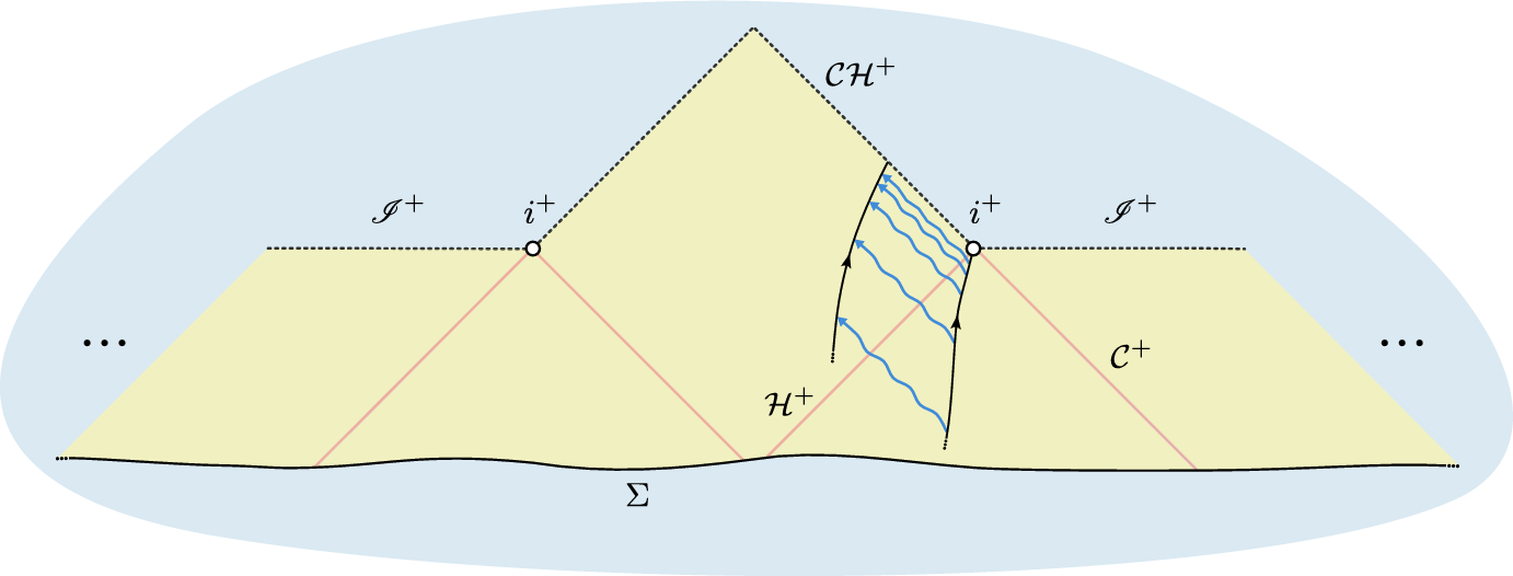
In this context, \(\mathcal \) corresponds to a region containing the event horizon and extending inside the dynamical black hole under investigation. In the course of the following proofs, we actually work with solutions defined in

$$\begin \mathcal \cap \, \end$$

for some \(v_1 \ge v_0\). We require (finitely many times) that the values of U and \(v_1\) are, respectively, sufficiently small and sufficiently large. A posteriori, this implies that our results hold in a region adjacent to both the event horizon and the Cauchy horizon of the dynamical black hole under investigation. We will highlight the steps where we constrain the values of U and \(v_1\). This occurs finitely many times and depends only on the \(L^\) norm of the initial data and possibly on \(\eta \), R (see Proposition 4.7), Y (see Proposition 4.12), and \(\varepsilon \) (see Proposition 4.13). These quantities can ultimately be chosen in terms of the initial data.

In this section, we are also going to prove that the apparent horizon

$$\begin \mathcal :=\ \end$$

is a non-empty \(C^1\) curve for large values of the v coordinate. It is also convenient to define the regular region

$$\begin \mathcal :=\, \end$$

which, as we will see, extends from the event horizon to part of the redshift region. The remaining part of the black hole interior is occupied by the trapped region

$$\begin \mathcal :=\. \end$$

(4.1)

For the system under analysis, the regular region is a priori non-empty, differently from the case of the Reissner–Nordström–de Sitter solution. In the latter case, indeed, every 2-sphere in the interior of the black hole region is a trapped surface and, furthermore, the apparent horizon coincides with the event horizon.

Remark 4.1

(on the main constants).

Throughout the bootstrap procedure, we use several auxiliary, positive quantities:

Redshift region (Proposition 4.7): \(\eta \), \(\delta = \delta (\eta )\), \(R = R(\delta )\),

No-shift region (Proposition 4.12): \(\varepsilon = \varepsilon (\beta )\), \(\Delta \), \(Y = Y(\Delta )\),

Early blueshift region (see (4.101)): \(\beta \).

We stress that, in Proposition 4.13, we choose \(\Delta \) in function of \(\varepsilon \). However, as explained in Remark 4.14, an analogous proof holds even if we choose \(\Delta \) independently from \(\varepsilon \). All above constants can be ultimately defined in terms of the initial data.

In particular, we have:

\(\delta \rightarrow 0\) as \(\eta \rightarrow 0\) and \(R \rightarrow r_+\) as \(\delta \rightarrow 0\) (see Proposition 4.7),

\(Y \rightarrow r_\) as \(\Delta \rightarrow 0\) (see Proposition 4.13),

\(\varepsilon \rightarrow 0\) as \(\beta \rightarrow 0\) (see Lemma 4.16).

4.1 Event Horizon

Recall that \(\varpi _+\), \(Q_+\) and \(\Lambda \) are the parameters of the final sub-extremal Reissner–Nordström–de Sitter black hole (see assumption (F)), while \(r_+\) and \(K_+\) denote the radius and the surface gravity, respectively, associated to its event horizon.

Proposition 4.2

(bounds along the event horizon).

For every \(v \ge v_0\), we have:

$$\begin 0 < r_ - r(0, v)&\le C_}e^, \end$$

(4.2)

$$\begin 0 < \lambda (0, v)&\le C_}e^, \end$$

(4.3)

$$\begin \frac}}} \le |\nu |(0, v)&\le C_} e^, \end$$

(4.4)

$$\begin |\varpi (0, v) - \varpi _+|&\le C_}e^, \end$$

(4.5)

$$\begin |Q(0, v) - Q_+|&\le C_} e^, \end$$

(4.6)

$$\begin |K(0, v) - K_+|&\le C_} e^, \end$$

(4.7)

$$\begin |\partial _v \log \Omega ^2(0, v) - 2K(0, v) |&\le C_} e^, \end$$

(4.8)

$$\begin |D_u \phi |(0, v)&\le C_} |\nu |(0, v) e^, &\textrm\,\, s < 2K_+, \\ C_} (v - v_0), &\textrm\,\, s = 2K_+,\\ C_}, & \textrm\,\, s > 2K_+, \end\right. } \end$$

(4.9)

$$\begin |\phi |(0, v) + |\partial _v \phi |(0, v)&\le C_} e^. \end$$

(4.10)

where \(C_}\) is a positive constant depending only on the initial data.

Proof

The proof exploits the decay due to the redshift effect, similarly to the proof of [80, proposition 4.4]. In the current case, however, the competition between the redshift effect and the exponential Price law is evident in the estimate for \(|D_u \phi |\) (see already Remark 4.3).

In the following, the letter C will denote a positive constant depending uniquely on the initial data. Moreover, we will exploit the assumptions (2.45) and (2.48) on \(\kappa \) and \(\nu \), respectively, multiple times in the next computations.

Preliminary bounds and exponential growth of \(\varvec\): first, we notice that (2.50) and (2.54) imply

$$\begin 0< r(0, v_0) \le r(0, v)< r_+ < + \infty , \quad \forall \, v \ge v_0. \end$$

(4.11)

It will also be useful to write (2.35), when evaluated on \(\mathcal ^+\), as

$$\begin \partial _v \log |\nu |(0, v) = 2K(0, v) - m^2 r(0, v) |\phi |^2(0, v). \end$$

(4.12)

Now, given \(\epsilon > 0\), expressions (2.49), (2.53) and the boundedness of r provide a sufficiently large \(v_1 > v_0\) such that

$$\begin \left| 2K(0, v) - m^2 r(0, v) |\phi |^2(0, v) - 2K_+ \right| < \epsilon , \quad \forall \, v \ge v_1. \end$$

(4.13)

This estimate will be improved during the next steps of the current proof, but for the moment we can use it in (4.12) and require \(\epsilon \) to be sufficiently small to obtain

$$\begin 0< K_+ < 2K_+ - \epsilon \le \partial _v \log |\nu |(0, v) \le 2K_+ + \epsilon , \quad \forall \, v \ge v_1, \end$$

(4.14)

and so, by integrating and due to (2.44):

$$\begin e^ \le |\nu |(0, v) \le e^, \quad \forall \, v \ge v_1. \end$$

(4.15)

Note that \(\Omega ^2(0, v) = -4 \nu (0, v)\) for every \(v \ge v_0\), by (2.19). So, (2.49), (4.12) and the boundedness of r entail

$$\begin \left| \partial _v \log \Omega ^2 (0, v) - 2K(0, v) \right| \le C e^. \end$$

To obtain (4.3), we first show that \(\frac\) admits a finite limit as \(v \rightarrow +\infty \), and that such a limit is zero. Indeed, by assumptions (A) and (F), we have that \(\lim _ \lambda (0, v) = \lim _ (1-\mu )(0, v) = 0\). Moreover, due to (4.15) and to the fact that \(\lambda _^+} > 0\):

$$\begin \lim _\frac(0, v) = 0. \end$$

(4.16)

Exponential decays: We now focus on the proof of the decay of \(\lambda \). Using (2.7) and (2.19) we cast one of the Raychaudhuri equations as

$$\begin \partial _v \left( }\right) = -r \frac. \end$$

Using the above, assumptions (2.49) and (2.54), and exploiting (4.11) and (4.16), we have:

$$\begin 0&< \lambda (0, v) = \nu (0, v) \int _^v \partial _v \left( }\right) (0, v') dv' \\&= \nu (0, v) \int _v^ \frac (0, v') dv' \le C \nu (0, v) \int _v^ \frac} dv' . \end$$

We now multiply and divide by \(K_+\), which is a positive quantity, and use that \(K_+ < \partial _v \log |\nu |(0, v')\) (see (4.14)), the fact that \(v \mapsto \nu ^(0, v)\) is an increasing function (indeed \(\partial _v \nu ^ = |\nu |^ \partial _v \log |\nu | > 0\)) and (4.15) to write

$$\begin \nu (0, v) \int _v^ \frac} dv'&\le \frac \int _v^ e^ \partial _v\left( }\right) (0, v')dv' \nonumber \\&\le C |\nu |(0, v)e^ \int _v^ \partial _v\left( }\right) (0, v')dv' = C e^, \end$$

(4.17)

which therefore gives \(0 < \lambda (0, v) \le C e^\) for every \(v \ge v_0\).

After recalling (2.51), we integrate (2.12) along the event horizon and use (4.11) and the exponential Price law (2.49) to write

$$\begin \left| Q(0, v) - Q_+ \right| = C \left| \int _v^ r^2(0, v') }(\phi \overline)(0, v') dv' \right| \le C e^, \quad \forall \, v \ge v_0.\nonumber \\ \end$$

(4.18)

This gives (4.6).

We can use this after integrating (2.26) (recall that \(\theta = r \partial _v \phi \)), together with (2.49), (2.52), (4.18), (4.11) and the decay of \(\lambda \) to see that

$$\begin |\varpi (0, v) - \varpi _+| \le Ce^, \quad \forall \, v \ge v_0, \end$$

(4.19)

therefore giving (4.5).

By integrating (4.17) and using (2.50), it also follows that

$$\begin 0 < r_+ - r(0, v) \le C e^. \end$$

Due to definition (2.34) and to the decays proved for Q and \(\varpi \), this is also sufficient to prove

$$\begin |K(0, v)-K_+| \le C e^, \quad \forall \, v \ge v_0. \end$$

(4.20)

This result also allows us to improve (4.13) and, following the same steps leading to (4.14) and (4.15), to obtain:

$$\begin |\nu |(0, v) \sim e^, \quad \forall \, v \ge v_0. \end$$

(4.21)

Bounds on \(\varvec\): we use (2.40), (2.49), (4.18) and (4.11) to write

$$\begin \left| \partial _v \left( \right) \right| (0, v) = \left| -\nu \partial _v \phi + m^2 \nu r \phi + i \frac \phi \right| (0, v) \le C|\nu |(0, v) e^.\qquad \nonumber \\ \end$$

(4.22)

Now, let us first assume that \(s < 2K_+\) and define the constant \(a :=K_+ - \frac > 0\). There exists \(V \ge v_0\), depending uniquely on the initial data, such that, using (2.35), (2.49) and (4.20), we obtain

$$\begin \partial _v \left( }\right) _^+} & = |\nu |(0, v) e^ \left( \right) \\ & > a |\nu |(0, v) e^, \end$$

for every \(v \ge V\). We can use this inequality when we integrate (4.22):

$$\begin |r D_u \phi |(0, v)&\le C\left( ^v |\nu |(0, v') e^ dv'}\right) \nonumber \\&< C\left( \int _^v \partial _v \left( }\right) dv'}\right) \nonumber \\&\le C \left( |\nu |(0, v)e^}\right) , \end$$

(4.23)

where we emphasize that C depends uniquely on the initial data. Using (4.21) and the boundedness of r, we conclude that

$$\begin |D_u \phi |(0, v) \le C |\nu |(0, v) e^ \lesssim e^, \quad \forall \, v \ge v_0, \end$$

when \(s < 2K_+\).

On the other hand, when \(s > 2K_+\), (4.21) gives:

$$\begin |r D_u \phi |(0, v) \le C\left( ^v e^ dv'}\right) \le \tilde, \end$$

for some \(\tilde\) determined by the initial data and for every \(v \ge v_0\). The final estimate follows from (4.11).

When \(s= 2K_+\), we can integrate (4.22) and use (4.21) to get

$$\begin |r D_u \phi |(0, v) \le C \left( ^v |\nu |(0, v') e^ dv'}\right) \le \tilde(v - v_0), \quad \forall \, v \ge v_0, \end$$

for some \(\tilde > 0\) depending on the initial data. The final estimate follows again from the boundedness of r.

Finally, (4.10) follows from (2.49). We then choose \(C_}\) as the largest of the previous positive constants depending on the initial data. \(\square \)

Remark 4.3

(Redshift effect).

From the point of view of a family of observers crossing the event horizon \(\mathcal ^+\), the energy associated to the null geodesics ruling \(\mathcal ^+\) decays as \(e^\) due to the redshift effect.

This is the same rate at which we found the geometric quantity \(\left| \nu ^ D_u \phi \right| \) to decay for \(s > 2K_+\) along the event horizon (see (4.9)). Here, the constant s is the same as in (2.49). For \(s < 2K_+\), the quantity \(\left| \nu ^ D_u \phi \right| \) decays as \(e^\) or faster, which is the same rate dictated by the Price law upper bound (2.49). From these two different rates, we deduce the physical relevance of two competing phenomena along the event horizon: the redshift effect and the decay of the scalar field \(\phi \).

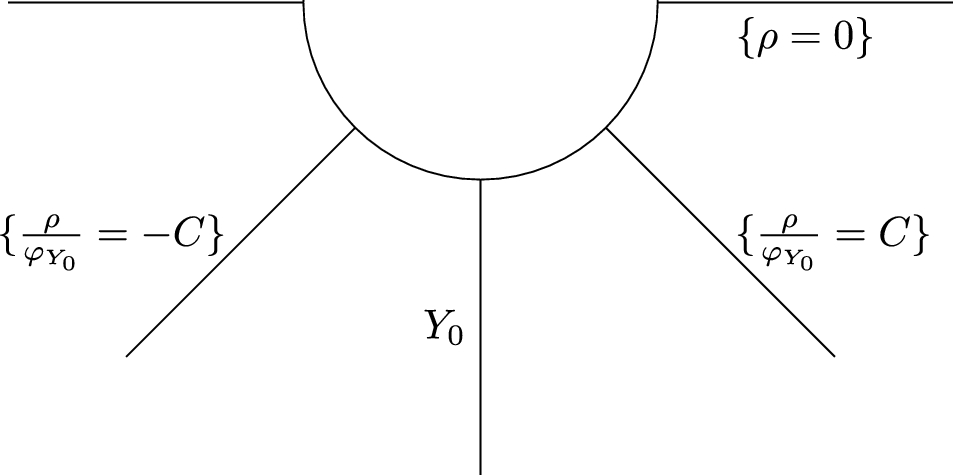
4.2 Level Sets of the Area-Radius Function

The strategy of the next proofs is based on a partition of the past set \(\mathcal \). In the two-dimensional quotient space that we are considering, such subsets are mainly separated by curves where the area-radius function is constant. We review the main properties of the sets

$$\begin \Gamma _ :=\\, :\, r(u, v) = \varrho \} \end$$

(4.24)

for some \(\varrho \in (0, r_+)\) (see also [19]).

Lemma 4.4

(properties of \(\Gamma _\)).

Assume that \(\Gamma _ \ne \varnothing \). Then, the following set equality holds:

$$\begin \Gamma _ = \(v), v) \, :\, v \in [v_1, +\infty ) \}, \end$$

for some \(v_1 \ge v_0\) and for some \(C^1\) function \(u_ :[v_1, +\infty ) \rightarrow \mathbb \) such that \(r(u_(\cdot ), \cdot ) \equiv \varrho \). Moreover, let

$$\begin \underline :=\inf \(v), v) \le 0 \}. \end$$

(4.25)

Then, the following properties are satisfied:

\(\varvec.}\) \(\Gamma _\) is a \(C^1\) curve,

\(\varvec.}\) We have

$$\begin u'_(v) = - \frac(v), v)}(v), v)}, \end$$

(4.26)

\(\varvec.}\) \(\lambda (u_(v), v) \le 0\) for every \(v \ge \underline\).

Lemma 4.5

(conditions to bound \(\lambda \) away from zero).

Let \(\varrho \in (r_, r_+)\). Assume that \(\Gamma _ \ne \emptyset \) and that for every \(\epsilon > 0\) there exists \(v_1 \ge v_0\) and \(c > 0\) such that

$$\begin |Q(u_(v), v) - Q_+| + |\varpi (u_(v), v) - \varpi _+| < \epsilon , \quad \forall \, v \ge v_1, \end$$

and

$$\begin 0 < c \le \kappa (u_(v), v) \le 1, \quad \forall \, v \ge v_1. \end$$

Then, there exist positive constants \(C_1\) and \(C_2\) such that:

$$\begin -C_2 \le \lambda (u_(v), v) \le - C_1 < 0, \quad \forall \, v \ge v_1. \end$$

Proof

Assume that \(\epsilon \) is sufficiently small. We then use (2.16) to write

$$\begin (1 - \mu )(u_\varrho (v), v)&= \left( \left( \right) -\frac\varpi _+ + \frac+\frac - \frac\varrho ^2}\right) (u_\varrho (v), v) \\&= (1-\mu )(\varrho , \varpi _+, Q_+) + O(\epsilon ), \end$$

for every \(v \ge v_1\). After inspecting the plot of \((1-\mu )(\cdot , \varpi _+, Q_+)\) (see, e.g., [17, section 3]), using the smallness of \(\epsilon \), (2.33) and the bounds on \(\kappa (u_(\cdot ), \cdot )\), we have:

$$\begin -C_2 \le \lambda (u_\varrho (v), v)=[\kappa (1-\mu )](u_\varrho (v), v) \le - C_1 < 0, \end$$

for some positive constants \(C_1\) and \(C_2\). \(\square \)

We use the definitions (4.1) and (4.25) of \(\mathcal \) and \(\underline\), respectively, for the next result.

Corollary 4.6

(entering the trapped region).

If the assumptions of Lemma 4.5 are satisfied, the curve \(\Gamma _\) is spacelike for large values of the v coordinate. Moreover, \(\underline < +\infty \) and \(\Gamma _ \cap \ \subset \mathcal \).

Proof

The conclusion follows from the negativity of \(\nu \) in \(\mathcal \) and of \(\lambda \) in \(\Gamma _ \cap \\), for some \(v_1 \ge v_0\) (see Lemma 4.5). \(\square \)

4.3 Redshift Region

For some fixed R, chosen close enough to \(r_+\) (see assumption (F)), we now study the region \(J^(\Gamma _R)\), after proving that it is non-empty.Footnote 24 We denote this set as the redshift region (see also [22, 61, 80]). Most of the estimates showed in Proposition 4.2 propagate throughout the redshift region, and the interplay between the decay of the scalar field and the redshift effect that we observed along the event horizon \(\mathcal ^+\) (see Remark 4.3) is still present.

To obtain quantitative bounds in this region, it is sufficient to bootstrap the estimates on \(|\phi |\), \(|\partial _v \phi |\), \(|D_u \phi |\), \(\kappa \) and \(|\nu |\) from \(\mathcal ^+\), and exploit these to achieve the remaining bounds. In particular, we employ the results of Proposition 4.2 and use the smallness of \(r_+ - r\) to close the bootstrap inequalities. The proof is an adaptation of the one in [80, proposition 4.5] to the case of exponential estimates. In particular, this requires a careful treatment of the Gronwall argument used to close the bootstrap for \(|D_u \phi |\). The estimates that we obtain depend on the integrable quantity \(u \Omega ^2(0, v) \sim u e^\) (see proposition 4.2).

Proposition 4.7

(propagation of estimates by redshift).

Given a fixed \(\eta \in (0, K_+)\), let \(\delta \in (0, \eta )\) be small compared to the initial data and to \(\eta \). Moreover, let R be a fixed constant such that

$$\begin 0< r_+ - R < \delta \end$$

and consider the function

$$\begin c(s) := s, & \text 0 < s \le 2K_+ - \eta , \\ 2K_+ - \eta , &\text s \ge 2K_+ - \eta . \end\right. } \end$$

(4.27)

Then, given \(v_1 \ge v_0\) large, whose size depends on the initial data, we have \(J^(\Gamma _R) \cap \ \ne \varnothing \). Moreover, for every \((u, v) \in J^(\Gamma _R) \cap \\), the following inequalities hold:

$$\begin 2\left( \right) \le u \Omega ^2(0, v)&\le C \delta , \end$$

(4.28)

$$\begin 0 < r_+ - r(u, v)&\le Ce^ + u \Omega ^2(0, v), \end$$

(4.29)

$$\begin |\lambda |(u, v)&\le Ce^ + u \Omega ^2(0, v), \end$$

(4.30)

$$\begin |\nu |(u, v)&\sim \Omega ^2(0, v), \end$$

(4.31)

$$\begin |\varpi (u, v) - \varpi _+|&\le C e^, \end$$

(4.32)

$$\begin |Q(u, v) - Q_+|&\le C e^, \end$$

(4.33)

$$\begin |K(u, v) - K_+|&\le C\left( + u\Omega ^2(0, v)}\right) ,\end$$

(4.34)

$$\begin | \partial _v \log \Omega ^2(u, v) - 2K(u, v) |&\le C e^, \end$$

(4.35)

$$\begin |D_u \phi |(u, v)&\le C |\nu |(u, v) e^, \end$$

(4.36)

$$\begin |\phi |(u, v) + |\partial _v \phi |(u, v)&\le C e^, \end$$

(4.37)

for a positive constant C that depends only on the initial data and on \(\eta \). Additionally, we have:

$$\begin \partial _u \lambda (u, v) < 0, \quad \forall \, (u, v) \in J^(\Gamma _R) \cap \. \end$$

(4.38)

Proof

In the following, \(C_}\) denotes the constant appearing in the statement of Proposition 4.2. We will use the notation

$$\begin C = C(N_}, \eta ) \end$$

to denote a positive constant depending on (a suitable norm of) the initial data of our IVP and on \(\eta \). We will use the same letter C to denote possibly different constants, when the exact expression of such constants is not important for the bootstrap. To close the bootstrap argument, we will require \(\delta \) to be sufficiently small with respect to \(N_}\) and \(\eta \). Moreover, we use that \(0 < \kappa \le 1\) and \(\nu < 0\) in \(\mathcal \) (see (3.4) and Remark 3.6) and that \(\lambda _^+} > 0\) (see assumption (G)) multiple times.

Setting up the bootstrap procedure: we recall that \(\mathcal \) is the maximal past set where we can define a solution to the characteristic IVP of Sect. 2.1, with initial data prescribed on \([0, U] \times \ \cup \ \times [v_0, +\infty )\). In the following, we consider \(v_1 \ge v_0\) to be sufficiently large with respect to the initial data and to \(\eta \), and define the set

$$\begin \mathcal _ :=\mathcal \cap \. \end$$

(4.39)

The latter is non-empty, since the area-radius function provides an increasing parametrization on \(\mathcal ^+\), and \(r(0, v) \rightarrow r_+\) as \(v \rightarrow +\infty \) (see (2.50) and (2.54)).

We now define \(\varvec\) as the set of points q in \(\mathcal _\) such that the following four inequalities hold for every (u, v) in \(J^(q) \cap \mathcal _\):

$$\begin |\phi |(u, v) + |\partial _v \phi |(u, v)&\le 4C_} e^, \end$$

(4.40)

$$\begin |D_u \phi |(u, v)&\le M|\nu |(u, v) e^, \end$$

(4.41)

$$\begin \kappa (u, v)&\ge \frac, \end$$

(4.42)

$$\begin \frac \Omega ^2(0, v) \le |\nu |(u, v)&\le \Omega ^2(0, v), \end$$

(4.43)

where \(M > 0\) is a constant depending uniquely on the initial data.

We notice that, since E is a past set by construction, inequalities (4.40)–(4.43) can be integrated along causal curves ending in (u, v) and starting from the event horizon or from the null segment \([0, U] \times \\).

Outline of the proof: in the following, we show that estimates (4.28)–(4.38) are valid in E and, at the same time, use this result to close the bootstrap and show that \(E = \mathcal _\). The conclusion then follows after proving that \(\varnothing \ne J^(\Gamma _R) \cap \ \subset \mathcal _\).

Closing the bootstrap: let us now fix \((u, v) \in E\). First, we stress that we have the following bounds on the area-radius function:

$$\begin 0< r(0, v)-r(u, v) \le r_+ -r(u, v) \le \delta , \\ r(u, v) > \frac, \\ r(u, v) < r_+, \end\right. } \end$$

(4.44)

due to (4.39), assumption (G) and by taking \(\delta < \frac\).

We notice that, by (4.44) and (4.43):

$$\begin \delta \ge r(0, v) - r(u, v) = \int _0^u |\nu |(u', v) du' \ge C u \Omega ^2(0, v). \end$$

(4.45)

In particular:

$$\begin u\Omega ^2(0, v) \le C \delta . \end$$

(4.46)

We stress that in [80] this relation was taken as the definition of the redshift region and, on the other hand, the bounds for r were derived. A similar computation and (4.2) yield

$$\begin r_+ - r(u, v) =r_+ -r(0, v) +r(0, v) -r(u, v) \le C e^ + u \Omega ^2(0, v).\quad \end$$

(4.47)

Now, we use (2.11) and bootstrap inequalities (4.40) and (4.41) to get

$$\begin |\partial _u Q|(u, v) \le C M C_} r^2(u, v) |\nu |(u, v)e^. \end$$

After integrating in u and using (4.44):

$$\begin |Q(u, v) - Q(0, v)| \le C M C_} \delta e^. \end$$

(4.48)

Then, by Proposition 4.2 and by (4.27):

$$\begin |Q(u, v) - Q_+| \le |Q(u, v) - Q(0, v)| + |Q(0, v) - Q_+| \le C(N_}, M) e^.\nonumber \\ \end$$

(4.49)

Furthermore, by integrating (2.37) and using (4.40), (4.44) and the above bound on Q, we obtain

$$\begin |r \lambda |(u, v) \le r_+ |\lambda |(0, v) + \left( }, \eta ) + O\left( }\right) }\right) \int _0^u |\nu |(u', v)du'. \end$$

The decay of \(\lambda _^+}\) proved in Proposition 4.2 and (4.43) yields

$$\begin |\lambda |(u, v) \le C e^ + u\Omega ^2(0, v), \end$$

(4.50)

for a positive constant \(C=C(N_}, \eta )\).

We can apply the latter bound, together with bootstrap inequalities (4.40)–(4.42) and with (2.19), to estimate \(\varpi \). Indeed, (2.38) gives

$$\begin |\partial _u \varpi |(u, v) \le C|\nu |(u, v)e^. \end$$

Thus, (4.44) and the bounds along the event horizon let us write

$$\begin |\varpi (u, v) - \varpi _+| \le |\varpi (u, v) - \varpi (0, v)| + |\varpi (0, v) - \varpi _+| \le C e^.\qquad \end$$

(4.51)

The definition of K (see (2.34)), together with bounds (4.44), (4.47), (