2.1 Summary of the Results of Ref. [5]

The RWN spacetime, with metric given by (1.6) and (1.7), is a solution to the Einstein–Maxwell(–Maxwell)Footnote 1 equations with electromagnetic Faraday tensor \(F = \text A\), where A is the one-form \(A = -\fracc\text t\). Therefore, in the conventional \((x^0 =ct, r, \theta , \phi )\) coordinates, the only nonzero component of A is \(A_0 = -\frac\). Hence, the only nonzero components of F are \(F_ = - F_ = \frac\).

In an electromagnetic spacetime, the Dirac equation for a point electron with mass \(m_}\), charge \(-e\), and anomalous magnetic moment \(\mu _a\) is given by (note that each term acting on \(\Psi \) has units of energy)

$$\begin \tilde^\mu (i\hbar c\nabla _\mu -e A_\mu )\Psi + \tfrac\mu _a \tilde^F_\Psi - m_}c^2 \Psi =0. \end$$

(2.1)

The anomalous magnetic moment term, \(\frac\mu _a\tilde^F_\), is the covariant generalization of the corresponding term in flat spacetime, see Sect. 4.2.3 in [32]. This is accomplished by setting \(\tilde^ = i \tilde^\mu \tilde^\nu \). In the following, we leave \(\mu _a\) as a parameter. Physically, the anomalous magnetic moment is measured in multiples of the Bohr magneton: \(\mu _a = - a \frac}c}\), where a is dimensionless. The first perturbative term in QED in flat spacetime gives \(a = \frac\alpha _}} \approx 0.00116\); cf. our discussion in the Sect. 1.

By multiplying the Dirac equation (2.1) by \(\gamma ^0\), we can recast it into a Hamiltonian form

$$\begin i \hbar \partial _t \Psi = H \Psi . \end$$

(2.2)

Due to the static nature of the spacetime, the operator H does not depend on time.

For each time t, let \(\Sigma _t\) denote the hypersurface of constant t within the \((t,r,\theta , \phi )\) coordinates. We define an inner product on \(\Sigma _t\) via

(2.3)

Here, \(\overline\) is the conjugate bi-spinor defined as \(\overline:= \Psi ^\dagger \gamma ^0\), n is the unit future directed timelike normal to \(\Sigma _t\), and \(dV__t}\) is the volume form on \(\Sigma _t\) induced from its Riemannian metric. This choice of inner product can be motivated from an action principle. It can also be motivated from the conservation of current density, i.e., \(\nabla _\mu j^\mu = 0\) where \(j^\mu = \overline\tilde^\mu \Psi \).

Thus, for each t, we have a Hilbert space

$$\begin \mathcal _t =\^4 \, \mid \,(\Psi ,\Psi )_ <\infty \}. \end$$

(2.4)

The operator H in (2.2) on the Hilbert space \(\mathcal _t\) is called the Dirac Hamiltonian on \(\Sigma _t\).

The spherical symmetry present within the Lorentzian metric and the electromagnetic field allows one to perform a separation of variables and decompose the Hilbert space \(\mathcal _t\) into a direct sum of partial wave subspaces [6], see also [32, Sect. 4.6]. The partial wave subspaces are indexed by a triplet \((j, m_j, k_j)\) where

$$\begin j = \frac, \frac, \frac \dotsc ; \quad m_j = -j, -j+1, \dotsc , j-1, j; \quad k_j = \pm \left( j + \frac\right) . \end$$

(2.5)

These correspond to certain eigenvalues of well-known operators on \(L^2(\mathbb ^2)^4\), see [32, p. 126]. The Dirac Hamiltonian H acting on each partial wave subspace is given by a two-dimensional reduced Hamiltonian (compare with [32, eq. (5.46)]):

$$\begin H_= \begin m_}c^2 f(r) - \frac & -\hbar c f^2(r) \partial _r + \hbar c f(r) \frac + \mu _af(r)\frac \\ \hbar c f^2(r) \partial _r + \hbar c f(r)\frac +\mu _a f(r) \frac & -m_}c^2 f(r) - \frac \end \end$$

(2.6)

which acts on the Hilbert space

$$\begin L^2\big ((0,\infty ), f(r)^dr\big )^2. \end$$

(2.7)

For a derivation of this form of the reduced Hamiltonian, see [6, p. 76] (see also [2]). Although each partial wave subspace depends on the triplet \((j,m_j, k_j)\), the reduced Hamiltonian \(H_\) only depends on the integer \(k_j\). (The independence of the reduced Hamiltonian on \(m_j\) is the reason for the degeneracy of the different spin states within the hydrogen atom; it is a consequence of spherical symmetry.)

The Dirac Hamiltonian H on \(\Sigma _t\) is essentially self-adjoint on the domain of \(C^\infty \) bi-spinors compactly supported away from the origin \(r = 0\) if and only if each reduced Hamiltonian \(H_\) is essentially self-adjoint on \(C^\infty _c(0,\infty )^2\), in which case, the spectrum of the corresponding self-adjoint operator (still denoted by H) is the union of the spectra of the self-adjoint operators for the reduced Hamiltonians (still denoted by \(H_\)). For a proof, see [32, Lem. 4.15] which generalizes to our setting. This reduces the problem to finding the spectrum for each reduced Hamiltonian.

The following theorem was proved in [5]. It says that essential self-adjointness is guaranteed for each reduced Hamiltonian \(H_\) provided the anomalous magnetic moment is not too small.

Theorem 2.1

(Belgiorno–Martellini–Baldicchi [5]). Each reduced Hamiltonian \(H_\) is essentially self-adjoint on \(C^\infty _c(0,\infty )^2\) if and only if \(|\mu _a| \ge \frac\frac\hbar }\), in which case the following hold for the self-adjoint Dirac Hamiltonian H:

(a)

The essential spectrum of H is \((-\infty , -m_}c^2] \cup [m_}c^2, \infty )\);

(b)

the purely absolutely continuous spectrum of H is \((-\infty , m_}c^2) (m_}c^2, \infty )\);

(c)

the singular continuous spectrum of H is empty;

(d)

H has infinitely many eigenvalues in the gap \((-m_}c^2, m_}c^2)\) of its essential spectrum.

Remark 2.2

Recall that the empirical anomalous magnetic moment is \(\mu _a = - a \frac}c}\), where a is dimensionless, see [12]. In first perturbative order, QED in flat spacetime gives \(a = \frac\alpha _}} \approx 0.00116\). With this classical value for the anomalous magnetic moment of the electron, the hurdle for essential self-adjointness is overwhelmingly cleared:

$$\begin \frac\frac\hbar }\frac}} = 6\pi \fracm_}}}}e} \,\approx \, 1.27\cdot 10^ \,\ll \, 1. \qquad \qquad \qquad \qquad \qquad \qquad \quad \square \end$$

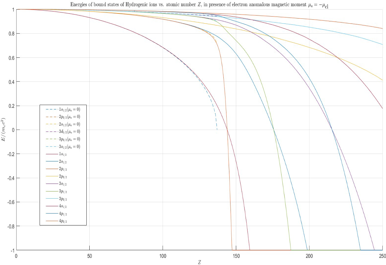
Theorem 2.1(d) implies that the discrete spectrum of the Dirac Hamiltonian on the RWN spacetime has infinitely many eigenvalues. In this paper, we rigorously investigate the discrete spectrum and classify it. We also wish to compare it to the discrete spectrum of the corresponding special-relativistic hydrogenic ion problem. A naturally tempting conjecture is that the discrete spectrum of the Dirac equation for an electron with anomalous magnetic moment in the RWN spacetime will converge to the discrete spectrum of the corresponding special-relativistic problem in the limit when Newton’s \(G\rightarrow 0\), given realistic values for the electron parameters. While we will not attempt to prove this conjecture in the present paper, we have carried out a numerical study of the eigenvalue problem which supports this conjecture.

2.2 Dimensionless Variables and Parameters

The conventional Gaussian units (or, for that matter, also the modern SI units) come equipped with numerical values that obscure the understanding of the Dirac equation for hydrogenic ions more than they illuminate it. It is advisable to switch to dimensionless quantities by choosing reference units that are more suitable to the atomic realm. Items 1 and 2 concern the RWN metric, items 3–4 concern Dirac’s equation.

1.

The replacement \(r \mapsto \frac}c} r\) renders r dimensionless and measures distance as multiple of the electron’s Compton wavelength. As a result, f(r) now reads

$$\begin f(r) = \sqrt}}\,\frac + \frac}^2Q^2}\,\frac}. \end$$

(2.8)

2.

The coefficients of \(\frac\) and of \(\frac\) in (2.8) are now themselves dimensionless parameters, and writing f(r) simply as

$$\begin f(r) = \sqrt + \frac}\, \end$$

(2.9)

defines \(A_*\) and \(Z_*\); note that the condition for a naked singularity becomes \(A_* < Z_*\).

The asymptotic behavior of \(1/f^2\) will be useful, so we record it here:

$$\begin \frac = \left\ Z_*^r^2 + O(r^3) & \text r \rightarrow 0 \\ & \, \\ 1 + O(r^) & \text r \rightarrow \infty . \end \right. \end$$

(2.10)

Remark 2.3

The motivation for our starred letters \(A_*\) and \(Z_*\) becomes obvious when comparing (2.8) with (2.9), by recalling that \(Q=Ze\) and \(M=:A(Z,N)m_}\), where \(m_}\) denotes the proton mass and A(Z, N) the nuclear mass number. This reveals that

$$\begin A_*&:= \mathcal \alpha _}}\frac}}}}A, \end$$

(2.11)

$$\begin Z_*&:= \sqrt}\alpha _}}Z, \end$$

(2.12)

where we have also introduced the dimensionless gravitational constant

$$\begin \mathcal :=Gm_}^2/e^2. \end$$

(2.13)

Remark 2.4

What we denote as \(A_*\) has been called the gravitational fine structure constant for the interaction of a particle of mass M with one of mass \(m_}\), see [17], but we prefer to reserve the name gravitational fine structure constant for that quantity when \(M=m_}\). \(\square \)

3.

We relabel \(k_j\) as k and define the operator \(K_k:=\frac}c^2}H_\).

4.

In order to facilitate the comparison of our results with those in [32], we also introduce \(\gamma := -Z\frac = -Z\alpha _}}\). Note that \(Z_* = -\sqrt} \gamma \).

5.

Recalling that \(\mu _a = -a\frac}c}\), with \(a = \frac}}}\) to first order in perturbative flat spacetime QED, where \(\alpha _}}\) is Sommerfeld’s fine structure constant, we now define \(\lambda := -\fraca \gamma \). With our choice of a, we have \(\lambda = \fracZ\alpha _}}^2\).

6.

For \(E \in (-m_}c^2, m_}c^2)\), define \(\varepsilon := \frac}c^2}\). Hence, \(\varepsilon \in (-1,1)\) is dimensionless. In some of the following proofs, \(\varepsilon = \pm 1\) will be considered even though it is not part of the discrete spectrum by Theorem 2.1.

With this new notation, the operator \(K_k\) becomes

$$\begin K_k = \begin f(r)+\frac & -f^2(r) \partial _ + f(r) \frac - f(r) \frac \\ f^2(r)\partial _ + f(r)\frac - f(r) \frac & -f(r)+\frac \end. \end$$

(2.14)

Remark 2.5

Note that f(r), given in (2.9), is the only place in \(K_k\) where Newton’s gravitational constant G, or for that matter its dimensionless version \(\mathcal \), enters, through \(A_*\) and \(Z_*\). Formally, the \(\mathcal \rightarrow 0\) limit yields \(f(r)\rightarrow 1\) for \(r>0\), and the reduced Hamiltonian (2.14) defined on its minimal domain \(C^\infty _c(0,\infty )^2\) becomes the reduced Hamiltonian in the corresponding special-relativistic problem, see [32, eq. (7.167))]. \(\square \)

2.3 The Prüfer Transformation

The eigenvalue problem for the reduced Hamiltonian yields a coupled system of differential equations. In this section, we use a Prüfer transformation to an equivalent system of two differential equations where one of them is decoupled from the other. This technique has been recognized in the past to help numerically solve eigenvalue problems for Dirac operators [35].

Note that E is an eigenvalue for \(H_\) if and only if \(\varepsilon \) is an eigenvalue for \(K_k\), where \(K_k\) is given by (2.14). The eigenvalue problem

$$\begin K_k \begin u \\ v \end = \varepsilon \begin u \\ v \end \end$$

(2.15)

yields the following coupled system of first-order linear differential equations

$$\begin&u'(r) + \frac\left( \frac - \frac\right) u(r) - \frac\left( f-\frac + \varepsilon \right) v(r) =0 \end$$

(2.16)

$$\begin&v'(r) - \frac\left( \frac - \frac\right) v( r) - \frac\left( f + \frac - \varepsilon \right) u(r) = 0. \end$$

(2.17)

We introduce the variables R(r) and \(\Omega (r)\) via a Prüfer transform:

$$\begin R(r) := \sqrt \quad \text \quad \Omega (r) := 2\arctan \left( \frac \right) , \end$$

(2.18)

where \(R \in [0, \infty )\) and \(\Omega \in (-\pi , \pi ]\). Then,

$$\begin u(r) \,=\ R \cos \left( \frac\Omega \right) \quad \text \quad v(r) = R \sin \left( \frac\Omega \right) . \end$$

(2.19)

Summing (2.16) \(\cdot u\) and (2.17) \(\cdot v\) gives

$$\begin \frac = \frac\sin \Omega + \frac\left( -\frac + \frac \right) \cos \Omega . \end$$

(2.20)

Likewise, summing (2.17)\(\cdot u\) and −(2.16) \(\cdot v\) gives

$$\begin \Omega ' = \frac\cos \Omega + \frac\left( \frac - \frac \right) \sin \Omega + \frac\left( \frac - \varepsilon \right) . \end$$

(2.21)

Although (2.16) and (2.17) is a linear system and (2.20) and (2.21) is nonlinear, the advantage we gain is that the equation for \(\Omega '\) does not depend on R. Therefore, we only need to study the differential equation (2.21) for \(\Omega \) and then R can be solved by integrating (2.20).

Once we solve for \(\Omega (r)\) and R(r), we can define u(r) and v(r) via (2.19). If u and v belong to the Hilbert space \(L^2\big ((0,\infty ), f(r)^dr^2\big )\), which holds if and only if \(R/f \in L^2\big ((0,\infty ), dr\big )\), then the corresponding wave function \(\Psi \) represents an element of the Hilbert space \(\mathcal _t.\)

2.4 Conversion to a Dynamical System on a Compact Cylinder

The study of (2.21) is facilitated by converting the differential equation into a dynamical system on a compact cylinder. First, we make the system autonomous by introducing a new differential equation, \(r' = 1\), so that r is now a dependent variable. However, the autonomous two-dimensional system, \(r' = 1\) and (2.21), is not compact and is singular at the origin \(r = 0\). We rectify both of these concerns. We introduce transformations that will make the system compact and remove the singularity at the origin \(r = 0\).

We first compactify the system by bringing \(r = \infty \) into a finite value. Introduce a new independent variable \(\eta \) via the transformation

$$\begin \eta : = T(r) := \frac \quad \text \quad r = T^(\eta ) = \frac. \end$$

(2.22)

T maps \((0,\infty )\) diffeomorphically onto (0, 1). From (2.9), we have

$$\begin f\big (r\big ) =:\fracg(\eta ), \end$$

(2.23)

where

$$\begin g(\eta ) = \sqrt. \end$$

(2.24)

Note that \(g(\eta )\) is always positive since we are in the naked singularity sector, \(A_* < Z_*\).

Similar to (2.10), we have

$$\begin \frac = \frac = \left\ \frac + O(\eta ^3) & \text \eta \rightarrow 0 \\ & \, \\ 1 + O(\frac) & \text \eta \rightarrow 1. \end \right. \end$$

(2.25)

The system, \(r' = 1\) and (2.21), becomes

$$\begin \left\ \eta ' & =\, (1-\eta )^2 \\ \Omega ' & =\, \frac\cos \Omega + \frac\left( k(1-\eta ) - \lambda \frac \right) \sin \Omega + \frac\big (\gamma (1-\eta )-\varepsilon \eta \big ). \end \right. \end$$

(2.26)

The system (2.26) is now precompact. It is not compact since, unless \(\lambda =0\), there is still a singularity at \(\eta = 0\). (The coefficient for the anomalous magnetic moment \(\lambda \) behaves like \(1/\eta \) as \(\eta \rightarrow 0\).)

Remark 2.6

The fact that \(\eta = 0\) is a regular point of this dynamical system when there is no anomalous magnetic moment term, is connected with the loss of essential self-adjointness for the Dirac Hamiltonian on the RWN background, first noted by [6], that was discussed in the Sect. 1.

To rectify this issue with (2.26), we introduce a new independent variable \(\tau \) via \(\tau := r + \log (r)\), so that \(\frac = \eta \). Multiplying \(\eta '\) and \(\Omega '\) by \(\eta \) in (2.26) and introducing the notation \(\dot = \frac\) and \(\dot = \frac\), the system becomes

$$\begin \left\ \dot & =\, \eta (1-\eta )^2 \\ \dot & =\, \frac \cos \Omega + \frac\big (k\eta (1-\eta ) - \lambda (1-\eta )^2 \big )\sin \Omega + \frac\big (\gamma (1-\eta ) - \varepsilon \eta \big ). \end \right. \end$$

(2.27)

The system (2.27) is now compact and free of singularities. Understanding the solutions to this system will be the main objective for the remainder of the paper.

Remark 2.7

We note that, in addition to the eigenvalue parameter \(\varepsilon \in (-1,1)\), the above dynamical system depends on three other continuous parameters: \(\lambda \in \mathbb \), representing the non-dimensionalized value of the electron anomalous magnetic moment, \(\mathcal \in \mathbb _+\), the non-dimensionalized universal constant of gravitation, and \(m_p/m_e\), the ratio of proton to electron rest mass (the latter two parameters are hiding inside the function g), as well as the two discrete parameters \(k\in \mathbb \) and \(Z \in \mathbb \). With so many parameters, one should expect the presence of different regions in the parameter space with significantly different qualitative behavior for the system, and a wealth of bifurcation phenomena. For example, setting \(\mathcal = 0\), i.e., in the case of Minkowski spacetime as the background, with \(f \equiv 1\) (and hence \(g(\eta ) = \eta \)), the system (2.27) is still not compactified. One would have to multiply \(\eta '\) and \(\Omega '\) in (2.26) by \(\eta ^2\) instead of \(\eta \). In this case, the independent variable, call it \(}\), would have to satisfy \(\frac}} = \eta ^2\). This implies that the equilibrium points at \(\eta =0\) will be non-hyperbolic, giving rise to qualitatively different local phase portraits from those studied below. As another example, the restriction \(\lambda \ge \fracZ_* = \frac}}Z}\sqrt}\) that we encountered in Theorem 2.1 and will see again in Theorem 2.8 is connected with the presence of a bifurcation curve in the \((\mathcal ,\lambda )\) plane. \(\square \)

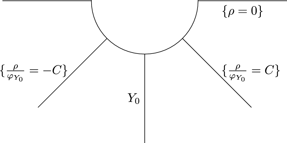
The system (2.27) now forms a dynamical system on the compact cylinder \(\mathcal = [0,1] \times \mathbb ^1\). There are only four equilibrium points. If we identify \(\mathcal \) with the fundamental domain \(\mathcal _* = [0,1] \times [-\pi , \pi )\), these four points are:

$$\begin S^- := (0,0), \quad N^- := (0,-\pi ), \quad S^+_\varepsilon := (1, -\arccos \varepsilon ), \quad N^+_\varepsilon := (1, \arccos \varepsilon ). \end$$

(2.28)

Note that \(S^-\) and \(N^-\) appear on the left boundary of the cylinder, while \(S^+_\varepsilon \) and \(N^+_\varepsilon \) appear on the right boundary of the cylinder. The Jacobians are

$$\begin J(S^-) = \begin 1 & \quad 0 \\ 0 & \quad -2\frac \end \quad&\text \quad J(N^-) = \begin 1 & \quad 0 \\ 0 & \quad 2\frac \end, \\ J(S^+_\varepsilon ) = \begin 0 & \quad 0 \\ c_+ & \quad \sqrt \end \quad&\text \quad J(N^+_\varepsilon ) = \begin 0 & \quad 0 \\ c_- & \quad -\sqrt \end, \end$$

where

$$\begin c_:= 2(1-A_* \pm k)\sqrt +2\varepsilon (2A_*-1) - 2\gamma . \end$$

\(S^-\) and \(N^-\) are hyperbolic equilibrium points; they correspond to a saddle and node, respectively. From the stable manifold theorem [27], there is a unique (up to translation by a constant) orbit emanating out of \(S^-\) into the cylinder, called the unstable manifold. \(S^+_\varepsilon \) and \(N^+_\varepsilon \) are non-hyperbolic equilibrium points, and so the stable manifold theorem does not apply. They correspond to saddle-nodes with the saddle part of \(S^+_\varepsilon \) pointing into the cylinder, and the saddle part of \(N^+_\varepsilon \) pointing out of the cylinder; see Theorem 1 in Sect. 2.11 of [27]. From Theorem 2.19 in [11], it follows that there is a unique (up to translation by a constant) orbit flowing into \(S^+_\varepsilon \) which will be referred to as its stable manifold.

A heteroclinic orbit is an orbit of the dynamical system whose \(\alpha \) and \(\omega \)-limit sets are equilibrium points. For the system (2.27), a heteroclinic orbit is one that begins and ends at the equilibrium points. Since \(\dot > 0\) for \(\eta \in (0,1)\), a heteroclinic orbit that does not lie on the boundary, \(\eta = 0\) or \(\eta = 1\), must connect one of the equilibrium points \(S^-\) or \(N^-\) to either \(S^+_\varepsilon \) or \(N^+_\varepsilon \); these will be referred to as non-boundary heteroclinic orbits. A non-boundary heteroclinic orbit that begins at \(S^-\) most likely ends at \(N^+_\varepsilon \). If, in the rare situation, a non-boundary heteroclinic orbit joins \(S^-\) to \(S^+_\varepsilon \), then the orbit will be called a saddles connector.

Theorem 2.8

Assume \(\lambda \ge \fracZ_*\). Consider a non-boundary heteroclinic orbit of the system (2.27). Then, this orbit represents an element of the Hilbert space, via (2.19), if and only if the orbit is a saddles connector.

Proof

As shown below (2.21), this orbit is an element of the Hilbert space if and only if \(R/f \in L^2\big ((0,\infty ), dr\big )\). From (2.20), we have

$$\begin R(r)= \exp \left( \int _^r\frac)})} d\tilde \right) \exp \left( \int _^r \frac)})}\left( -\frac} + \frac^2} \right) d\tilde\right) \end$$

for some \(r_0 \in (0, \infty )\). We first examine the \(L^2\) condition for the left end of the cylinder, \(\eta = 0\) (i.e., \(r = 0\)). Using (2.10) in the above expression for R(r), we conclude that

(i)

If the orbit begins at \(S^-\), then \(R(r) \propto r^ + o(1)\) as \(r \rightarrow 0\).

(ii)

If the orbit begins at \(N^-\), then \(R(r) \propto r^ + o(1)\) as \(r \rightarrow 0\).

Therefore, \(R^2(r)/f^2(r) \propto r^ + o(1)\) as \(r \rightarrow 0\). The \(L^2\) condition is satisfied in a neighborhood of \(r = 0\) if and only if \(2 \pm 2\lambda /Z_* > -1\). Therefore, (i) implies the \(L^2\) condition in a neighborhood of \(r = 0\), while (ii) does not so long as \(\lambda \ge \fracZ_*\).

Now, we examine the \(L^2\) condition for the right end of the cylinder, \(\eta = 1\) (i.e., \(r = \infty \)). Fix \(\alpha > 0\) such that \(\alpha < \sqrt\). Set \(\beta _:= \sqrt \pm \alpha > 0\). If the orbit ends at \(S^+_\varepsilon \), then \(\sin \Omega /f = -\sqrt + o(1)\) as \(r \rightarrow \infty \). Therefore, there is an \(R_\alpha \) such that \(\sin \Omega (r)/f(r)<-\beta _-\) whenever \(r>R_\alpha \). Using similar estimates for \(\cos \Omega /f\), we observe:

(iii)

If the orbit ends at \(S^+_\varepsilon \), then for some constants \(c_1\) and \(c_2\), we have the following:

In either case, the \(L^2\) condition is satisfied for \(R^2/f^2\) in a neighborhood of \(r = \infty \).

(iv)

If the orbit ends at \(N^+_\varepsilon \), then \(\sin \Omega /f = \sqrt + o(1)\) as \(r \rightarrow \infty \). Hence, R(r) exhibits exponential growth as \(r \rightarrow \infty \) and so the \(L^2\) condition is never satisfied. \(\square \)

Remark 2.9

If we instead considered negative values of \(\lambda \) in Theorem 2.8, then \(N^-\) and \(S^-\) would have switched roles and we would have required \(|\lambda | \ge \fracZ_*\). The assumption \(|\lambda | \ge \fracZ_*\) is equivalent to the assumption \(|\mu _a| \ge \frac\frac\hbar }\), which appeared in Theorem 2.1. In fact Theorem 2.8 offers another proof of the fact that H is essentially self-adjoint if and only if \(|\mu _a| \ge \frac\frac\hbar }\), see [32, Thm. 4.16]. \(\square \)

2.5 Proof of the Main Result

In this section, we will always assume the following conditions on our parameters

$$\begin Z_* \,>\,0, \quad \quad 0 \le A_* < Z_*\, \quad \quad \lambda \ge \fracZ_*. \end$$

Recall that the second assumption implies \(g(\eta ) > 0\) (naked singularity sector), and the last assumption guarantees essential self-adjointness. Also, the other parameter is k which is a nonzero integer. Lastly, recall that \(\gamma \) and \(Z_*\) are not independent parameters but are related via \(Z_* = -\sqrt}\gamma \) where \(\mathcal \) is given by (2.13).

Given Theorem 2.8, we wish to obtain saddles connectors for our system, which is our main result, Theorem 2.24, at the end of this section. We will follow the strategy first laid out in [20] and generalized in [19]; the latter will be our primary reference. Our compact dynamical system on the cylinder \(\mathcal = [0,1] \times \mathbb ^1\) is given by

$$\begin \left\ \dot & =\, }(\eta ) \\ \dot & =\, \mathfrak _\varepsilon (\eta , \Omega ). \end \right. \end$$

(2.29)

where \(\mathfrak (\eta )\) and \(\mathfrak _\varepsilon (\eta , \Omega )\) are given by the right hand sides of (2.27).

So long as \(-1< \varepsilon <1\), the dynamical system \(\mathcal \) satisfies properties (a)–(e) in Sect. 3.1 of [19] with \(x = \eta \), \(y = \Omega \), parameter \(\mu = \varepsilon \), and fundamental domain \(\mathcal _* = [0,1] \times [-\pi , \pi )\).

We briefly state these properties in our context.

(a):

\(F(0) = F(1) = 0\) and \(\mathfrak (\eta ) > 0\) for all \(\eta \in (0, 1)\). Consequently, equilibrium points can only occur at the boundary of the cylinder (i.e., at \(\eta = 0,1\)), and the boundaries \(\eta = 0\) and \(\eta = 1\) are images of orbits of the dynamical system. An orbit whose image is not completely contained in one of the boundaries \(\eta = 0\) or \(\eta = 1\) will be referred to as a non-boundary orbit. Since \(\mathfrak (\eta ) > 0\) for \(\eta \in (0, 1)\), the flow of the dynamical system “points to the right.” That is, for any non-boundary orbit \(\big (\eta (\tau ), \Omega (\tau )\big )\), we have \(\eta (\tau )\) is strictly increasing in \(\tau \).

(b):

\(S^-\) and \(N^-\), from (2.28), are hyperbolic equilibrium points; they correspond to a saddle and node, respectively. \(S^+_\varepsilon \) and \(N^+_\varepsilon \) are non-hyperbolic equilibrium points. We will let \(\mathcal ^-_\varepsilon \) and \(\mathcal ^+_\varepsilon \) denote the unstable and stable manifolds associated with \(S^-\) and \(S^+_\varepsilon \), respectively. Note that \(\mathcal ^-_\varepsilon \) and \(\mathcal ^+_\varepsilon \) coincide coincide when the orbit is a saddles connector.

(c):

Set \(\mathcal _* = [0, 1] \times [-\pi ,\pi )\) to be a fundamental domain of the universal cover \(\widetilde} = [0, 1] \times \mathbb \). The equilibrium points \(N^+_\varepsilon \) and \(S^+_\varepsilon \) stay within this fundamental domain for all \(\varepsilon \in (-1,1)\) and \(N^+_\varepsilon \) is always “above” \(S^+_\varepsilon \), that is, \(-\pi \le -\arccos \varepsilon< \arccos \varepsilon < \pi .\)

(d):

For all \((\eta ,\Omega ) \in \mathcal \), we have \(\frac\mathfrak _\varepsilon (\eta ,\Omega ) \le 0\).

(e):

Every non-boundary orbit is a heteroclinic orbit. That is, the \(\alpha \) and \(\omega \)-limit sets of any non-boundary orbit are precisely one-point sets containing equilibrium points on the boundary \(\eta = 0\) and \(\eta = 1\), respectively. Therefore, we will refer to the \(\alpha \) and \(\omega \)-limit sets as \(\alpha \) and \(\omega \)-limit points.

Only property (e) requires some justification. A quick calculation shows that Proposition 3.16 from [19] holds for \(\varepsilon \in (-1,1]\). (Note that \(\varepsilon \) is analogous to E in [