In the following we assume that (M, g) is a connected n-dimensional spacetime (time-oriented, oriented Lorentzian manifold). We assume further that M has a real analytic atlas with respect to which the metric g is real analytic. The purpose of the metric g is twofold. It provides an analytic volume form which is needed to identify functions with distributions. Secondly, it provides a causal structure in the form of a bundle of light cones. In principle it is not strictly necessary to derive these structures from a metric, but we assume so here for simplicity of the presentation.

We briefly explain the notations, assuming the signature convention is \((+,-,\ldots ,-)\). First, for a point \(x \in M\) we denote by \(V_x \subseteq T^*_x M\) the closed light cone in cotangent space with respect to the metric g, i.e., the set of covectors \(\xi \in T^*_x M\) with \(g^(\xi ,\xi ) \ge 0\). Then \(V_x \\) is the disjoint union of the future/past light cone \(V_x^\pm \). A covector \(\xi \in T^*_x M\) is called causal if it is in \(V_x \\). A causal covector is called future directed if it is contained in \(V_x^+\). We write \(V^\pm \) for the corresponding bundles, i.e., \(V^\pm = \sqcup _x V_x^\pm \). Therefore, \((x,\xi ) \in V^+\) will mean that \(\xi \) is a future directed causal covector. Recall that \(T^*(M \times \ldots \times M)\) is canonically isomorphic to \(T^*M^m\) and we will write typical elements as \((x_1,\xi _1,\ldots ,x_m,\xi _m)\).

4.1 Quantum Field Theory

A quantum field theory on (M, g) will be defined as an operator-valued distribution \(\Phi \), which we will call the field. To be more precise, let \(\mathcal \) be a Hilbert space with a dense set D. Then \(\Phi \) is a map \(\Phi : C^\infty _0(M) \rightarrow \textrm(D)\) such that \(f \mapsto \Phi (f) v\) is continuous for every \(v \in D\). The operator \(\Phi (f)\) can be unbounded. It is referred to as the smeared out field. One requires that \(\Phi (f)\) is symmetric on D if f is real-valued. We will assume for convenience and without loss of generality that D is complete with respect to the locally convex topology induced by the family of semi-norms

$$\begin p_(\phi ) = \Vert \Phi (f_1) \cdots \Phi (f_m) \phi \Vert , \end$$

where \(m \in \mathbb _0\) and \((f_1,\ldots ,f_m)\) is an arbitrary m-tupel of compactly supported smooth functions. We refer to this locally convex topology as the graph topology, as it is generated by the graph norms of all the elements of the algebra. Since the adjoints are densely defined the operators \(\Phi (f_1) \cdots \Phi (f_m)\) are closable. Therefore, one can always pass to the completion of the domain, which is then still contained in \(\mathcal \).

Given a spacetime region \(\mathcal \subseteq M\) one can form the \(*\)-algebra \(\mathcal (\mathcal )\) generated by the elements \(\Phi (f), f \in C^\infty _0(\mathcal )\). In case \(\Phi (f)\) is essentially self-adjoint for any real-valued \(f \in C^\infty _0(\mathcal )\) one can then consider the weak-\(*\)-closure of the set of all bounded operators generated by the spectral projections of \(\Phi (f)\). By von Neumann’s bi-commutant theorem, this algebra can be characterized as

$$\begin \mathcal (\mathcal ) = \(\mathcal ) \mid \forall f \in C^\infty _0(\mathcal ), A \text \Phi (f) \}'. \end$$

Here \(\mathcal ' = \(\mathcal ) \mid \forall A \in \mathcal , A B = B A\}\) as usual is the commutant of \(\mathcal \). Recall that a bounded operator A commutes with a self-adjoint operator T if and only if \(A T = T A\) as an inequality of unbounded operators with equality of domains. In particular, A leaves the domain of T invariant. If T is essentially self-adjoint on a dense set \(D \subseteq \mathcal \) then an operator \(A \in \mathcal (\mathcal )\) commutes with T therefore if and only if for all \(v,w \in D\) we have \(\langle T w, A v \rangle = \langle w,A T v \rangle \).

For a general symmetric unbounded operator T defined on a dense set D, we turn this into a definition and say a bounded operator \(A \in \mathcal (\mathcal )\) commutes (weakly) with T if for all \(v,w \in D\) we have \(\langle w, A\, T v \rangle = \langle T w, A\, v \rangle \). The set of operators commuting with T is then a set that is invariant under the map \(*\). It is called the weak commutant of T. It is easy to see that if A commutes with T then it also commutes with its closure. It is therefore sufficient to check commutation on a subset of the domain that is dense in the graph norm, so that the closure of the operator on this subset coincides with the operator. It is not sufficient to check this on a dense subset of the domain. As an example, consider the Laplace operator \(\Delta \) on the real line and the Laplace operator \(\Delta _D\) on the real line with Dirichlet boundary conditions at the point \(x=0\). If we take \(T = \Delta \) and \(A=(-\Delta _D+1)^\), then T and A do not commute. However, we have the relation \(\langle w, A\, T v \rangle = \langle T w, A\, v \rangle \) for all v, w in the dense set of smooth compactly supported functions that vanish to infinite order at the point 0. The reason is here that \(\Delta \) and \(\Delta _D\) restrict to the same operator on this space of functions, but the self-adjoint extensions are completely different. This shows that one has to consider domain issues carefully when using this definition and associated conclusions. For the functional analytic details, we refer to [25] as well as [8] for a discussion in the context of quantum field theory.

The von Neumann algebra (weakly) associated with the algebra generated by \(\Phi (f), f \in C^\infty _0(\mathcal )\) is then defined by

$$\begin \mathcal (\mathcal ) = \(\mathcal ) \mid \forall (f \in C^\infty _0(\mathcal ), v,w \in D), \langle w, A\, \Phi (f) v \rangle = \langle \Phi (\overline) w, A\, v\rangle \}'. \end$$

In this way every quantum field defines a net of von Neumann algebras, i.e., a von Neumann algebra \(\mathcal (\mathcal )\) associated to every spacetime region \(\mathcal \). Due to the nature of the weak commutant there are further technical conditions that ensure that this is again a local net, i.e., that it satisfies Einstein causality and the algebras of causally separated regions commute. We will, however, not discuss this here any further but refer to [11] for a detailed discussion of this in the context of Wightman fields on Minkowski space.

We now discuss a mild assumption about the quantum field.

4.2 Physical Conditions on States

Whereas on a curved spacetime there is no meaningful notion of momentum and energy and hence no preferred vacuum state, the notion of energy momentum should still exist in an asymptotic sense as a scaling limit. The notion of uniform microsupport for test functions is extremely well suited to capture this. On physical grounds one expects from a reasonably passive state \(\Omega \) to not allow for non-physical energy transfer. Assume that \((f_h)\) localizes in phase space to a point \((x,\xi )\) as \(t \searrow 0\). For the moment we also allow families \((\phi _h)\) of states in D describing an asymptotic physical situation. We think of \(\phi _h\) as a physical configuration that may become singular as \(h \searrow 0\). In QFT we then expect the following behavior depending on where in \(T^*M\) the point \((x,\xi )\) is localized. If \((x,\xi ) \in V^-\) we expect the state \(\Phi (f_h) \Omega \) to have added energy momentum \(-h^ \xi \) near x in an asymptotic sense. If \((x,\xi ) \in V^+\) we expect the operator \(\Phi (f_h)\) to erase the energy momentum \(h^\xi \) near x from the state \(\phi _h\). A state \(\Omega \in D\) not asymptotically carrying energy should not allow for asymptotic energy extraction. Hence, \(\Phi (f_h) \Omega \) should be exponentially small if \((x,\xi ) \notin V^-\).

The mathematically precise statement depends on the space of test functions employed and we would like to consider two versions.

4.3 Fields Defined on Compactly Supported Smooth Test Functions

Recall that \(C^\infty _(M)\) is the space of families of test functions that are uniformly exponentially small away from any neighborhood of the zero section in \(T^*M\). Given \((q_,\ldots ,q_) \in C^\infty _(M)\) we expect intuitively that the state \(\Phi (q_)\ldots \Phi (q_) \Omega \) contains no asymptotically extractable energy. We therefore should have that

$$\begin \Phi (f_h)\Phi (q_)\ldots \Phi (q_) \Omega \end$$

is exponentially small if \(f_h\) microlocalizes uniformly at a point \((x,\xi ) \notin V^-\). This motivates the following definition.

Definition 4.1

A vector \(\Omega \in D\) is called analytic if the following holds. If \(f_h \in C^\infty _(M)\) is microlocally uniformly supported in a compact set \(K \subset T^*M\) with \(K \cap V^- = \emptyset \) then, for all families \((q_),\ldots ,(q_) \in C^\infty _(M)\), we have the bound

$$\begin \Vert \Phi (f_h) \Phi (q_)\ldots \Phi (q_) \Omega \Vert \le C e^} \end$$

for some \(C>0, \delta >0\).

The subspace of analytic vectors will be denoted by \(D_a \subset D\).

Using Proposition 2.5 the above condition can be completely paraphrased in terms of analytic wavefront sets.

Proposition 4.2

A vector \(\Omega \in D\) is analytic if and only if for all \(n \in \mathbb \) the Hilbert space-valued distribution \(\Phi (\cdot ) \ldots \Phi (\cdot ) \Omega \) on \(M^n\) defined by

$$\begin f_1 \otimes \cdots \otimes f_n \mapsto \Phi (f_1) \ldots \Phi (f_n) \Omega \end$$

has its analytic wavefront set contained in the set of nonzero covectors \((x_1,\xi _1,\ldots x_n,\xi _n)\) satisfying for all \(1 \le k \le n\) that

$$\begin (\text \xi _j=0 \text j>k ) \text \xi _k \in V^+, \end$$

In other words, the first nonzero covector from the right must be future directed and causal.

Proof

That the wavefront set condition for \(k=1\) implies analyticity is a direct consequence of Proposition 2.5. We therefore only need to show that analyticity implies the analytic wavefront set condition for any \(1 < k \le n\). To show that the wavefront set condition is satisfied, it is sufficient, again by Proposition 2.5, to show that for families \(f_, \ldots f_ \in C^\infty _(M)\) with the properties

\((f_)\) is uniformly microsupported in a compact set of positive distance to \(V^-\),

\((f_) \in C^\infty _(M)\) for all \(j >k\),

we have that the family of vectors \( \Phi (f_)\cdots \Phi (f_) \Phi (f_) \Phi (f_) \cdots \Phi (f_) \Omega \) is exponentially small in the norm as \(h \searrow 0\). This is equivalent to

$$\begin&\langle \Phi (f_)\ldots \Phi (f_) \Phi (f_)\ldots \Phi (f_) \Omega , \Phi (f_)\ldots \Phi (f_) \Phi (f_) \ldots \Phi (f_) \Omega \rangle \\&\quad = \langle \Phi (\overline})\ldots \Phi (\overline}) \Phi (f_)\ldots \Phi (f_) \Phi (f_) \ldots \Phi (f_) \Omega , \\&\qquad \Phi (f_) \ldots \Phi (f_) \Omega \rangle \end$$

being exponentially small. Since the family of test functions

$$\begin \overline} \otimes \cdots \otimes \overline} \otimes f_ \otimes \cdots \otimes f_ \otimes f_ \otimes \cdots \otimes f_ \end$$

is polynomially bounded, the Cauchy–Schwarz inequality shows that exponential smallness is implied by exponential smallness of the family

$$\begin \Phi (f_) \ldots \Phi (f_) \Omega . \end$$

By Proposition 2.5 exponential smallness of this vector as \(h \searrow 0\) is a consequence of analyticity. \(\square \)

For a realistic quantum field, we expect the set \(D_a\) to be dense in the Hilbert space and in the domain of the field in the following sense. For every \(v \in D\) there exists a sequence \(v_n \in D_a\) such that for all \( f_1,\ldots ,f_m \in C^\infty _0(M)\) we have in the Hilbert space norm

$$\begin v_n \rightarrow v, \text \Phi (f_1)\ldots \Phi (f_m) v_n \rightarrow \Phi (f_1)\ldots \Phi (f_m) v. \end$$

This means that \(D_a\) is a dense subset in each of the domains of \(\Phi (f_1)\ldots \Phi (f_m)\) with respect to the graph norm.

Remark 4.3

We note that whereas we assume that D is invariant under \(\phi (f)\) this cannot be assumed for \(D_a\), as this is not compatible with Einstein causality. To illustrate this, we restrict this discussion to bosonic fields, for which the fields commute at spacelike separation. Assume \(\phi \) was a vector in \(D_a\) such that \(\Phi (f) \phi \in D_a\) for all \(f \in C^\infty _0(M)\). Then the distribution \([\Phi (\cdot ), \Phi (f)] \phi \) vanishes in the causal complement of the support of f and has its analytic wavefront set in \(V^+\). Since \(V^+\) is one-sided, this distribution has the unique continuation property and must therefore vanish (c.f. Proposition D.2). It follows that \([\Phi (\cdot ), \Phi (f)] \phi \) vanishes. Since this is true for all f with sufficiently small support it follows for all compactly supported f. Hence, \([\Phi (f_1), \Phi (f_2)] \phi =0\) for all test functions \(f_1, f_2 \in C^\infty _0(M)\). The existence of the dense and invariant set of analytic vectors therefore implies that the field algebra is commutative.

To keep the notations short, we write \(\mathcal \) for the algebra generated by \(\Phi (f), f \in C^\infty _0(M)\). Given an open set \(\mathcal \subseteq M\) we write \(\mathcal (\mathcal )\) for the algebra generated by \(\Phi (f), f \in C^\infty _0(\mathcal )\). Recall that a vector \(\phi \in D\) is called cyclic for an algebra of operators \(\mathcal \) on D if the set \(\mathcal \phi \) is dense in \(\mathcal \). In Minkowski theories, one usually assumes that the vacuum \(\Omega \) is a cyclic vector for the field algebra, and in fact that \(\mathcal \Omega \) is dense in D with respect to the graph topology. It is also natural to assume that there are many vacuum-like states \(\Omega \in D_a\) in the sense that there is a dense set of cyclic analytic vectors.

The existence of an analytic vector \(\Omega \in D_a\) with \(\mathcal \Omega \) being dense in D with respect to the graph topology is one of the weaker conditions one can make, and it readily implies two important properties of the quantum field: the Reeh–Schlieder property and the timelike tube property. The Reeh–Schlieder property means that the vector \(\Omega \) is a cyclic vector for the local algebra \(\mathcal (\mathcal )\) for any non-empty open \(\mathcal \subset M\). The timelike tube property is that the local von Neumann algebra \(\mathcal (\mathcal )\) of region \(\mathcal \) coincides with the local von Neumann algebra of a potentially much bigger region, \(\mathcal _T(\mathcal )\), the timelike hull of \(\mathcal \). We will state the precise theorems in Sect. 5.1.

We will see below that in case the theory satisfies a certain temperedness assumption the existence of a cyclic tempered analytic vector implies that there is a dense set of tempered analytic vectors.

4.4 Tempered Fields

In Minkowski space a good choice of test function space is the space of Schwartz functions \(\mathcal (\mathbb ^d)\). This space is particularly suited for spectral considerations as it contains the space \(\mathcal (C^\infty _0(\mathbb ^d))\) of functions that are localized in momentum space. Moreover, this space treats configuration and momentum space on an equal footing.

To define an analogue of Schwartz space on a general analytic manifold (M, g), one needs to specify some extra structure such as a special coordinate chart near infinity. We will choose here a more flexible path, by embedding the spacetime analytically into \(\mathbb ^\).

Any real analytic manifold (M, g) can be analytically embedded into \(\mathbb ^\) in such a way that the embedding is proper (see [17]). Given such an embedding, and restricting the space of functions to \(M \subset \mathbb ^\), we can define Schwartz spaces and spaces of analytic functions on a general real analytic manifold. In the following we fix a proper analytic embedding \(\iota : M \rightarrow \mathbb ^\). We denote by \(\mathcal (M)\) the space \(\iota ^*(\mathcal (\mathbb ^))\) of the restrictions of Schwartz functions. We equip \(\mathcal (M)\) with the natural quotient topology. The resulting topology is stronger than the \(C^\infty (M)\)-topology of uniform convergence of all derivatives on compact subsets. We have now constructed nuclear Frechét space \(\mathcal (M)\) in which \(C^\infty _0(M)\) is dense. Of course, also \(\mathcal _a(M) = \iota ^*(\mathcal (C^\infty _0(\mathbb ^))\) is dense in \(\mathcal (M)\). This space is subspace of the space of real analytic Schwartz functions that arise from restrictions of entire functions to M.

It is worth noting that the map \(}: \mathbb ^d \rightarrow \mathbb ^d\) defined as

$$\begin }(x_1,\ldots ,x_) = (x_1 \exp (x_1^2),\ldots , x_ \exp (x_^2)) \end$$

is also a proper analytic embedding and the pull-back \(\iota ^*\mathcal (\mathbb ^d)\) then consists of exponentially decaying real analytic functions. This means the embedding can always be modified so that \(\mathcal (M)\) consists of extremely fast decaying functions.

For Schwartz functions a uniform notion of localization at the zero section can be defined as follows. We say \(f_h \in \mathcal _(\mathbb ^d)\) if \(f_h\) microlocalizes uniformly away from any tubular neighborhood of the form \(\^ \times \mathbb ^d \mid \Vert \xi \Vert < \epsilon \}, \epsilon >0\). Now define \(\mathcal _(M) = \iota ^* \mathcal _(\mathbb ^)\) and \(\mathcal _a(M) = \iota ^*\mathcal _(\mathbb ^)\) by restriction. This definition is well behaved under various canonical constructions.

In case \(d'>d\) we have for the standard embedding \(\iota : \mathbb ^d \rightarrow \mathbb ^, (x_1,\ldots ,x_d) \mapsto (x_1,\ldots ,x_d,0,\ldots ,0)\) that \(\iota ^* \mathcal _(\mathbb ^) = \mathcal _(\mathbb ^)\).

If N is closed (compact without boundary), then \(\mathcal _(N)\) is independent of the embedding and equal to \(C^\infty _(N)\).

The notion of \((f_h) \in C^\infty _(M)\) is defined with respect to local analytic coordinates, whereas the notion of \((f_h) \in \mathcal _(M)\) is defined relative to an analytic embedding. However, for families \((f_h) \in C^\infty _(M)\) we have \((f_h) \in \mathcal _(M)\) if and only if \((f_h) \in C^\infty _(M)\). Hence, the notions by analytic coordinates and by embeddings coincide. In particular, this also implies that the dependence of the space \(\mathcal _(M)\) on the embedding disappears upon restriction to \(C^\infty _(M)\). The main purpose of the embedding is thus to control the microlocal properties of the functions near infinity.

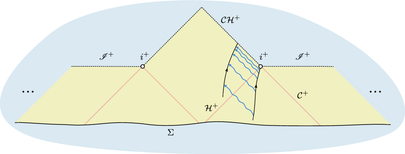
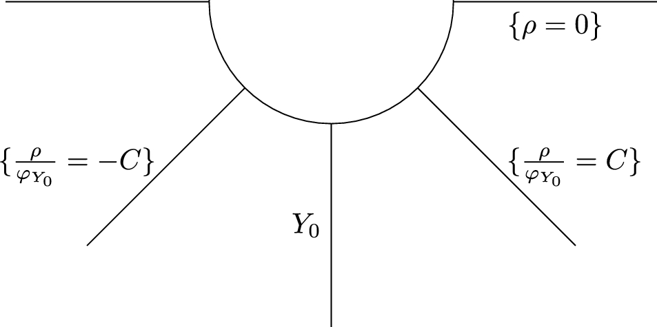
Example 4.4

The Schwarzschild–Kruskal spacetime is a four-dimensional analytic spacetime which is analytic-diffeomorphic to \(\mathcal \times \mathbb ^2\), where \(\mathcal \) is the region \(\^2 \mid T^2 - X^2<1\}\) in \(\mathbb ^2\). The equation

$$\begin T^2 - X^2 = \left( 1-\frac\right) e^} \end$$

implicitly defines a function r(T, X). Then the metric is given by

$$\begin g = \frac e^}(\textrmT^2 - \textrmX^2) - r^2 g_^2}. \end$$

The above description is called the Kruskal–Szekerez coordinate system. We can embed this spacetime analytically in \(\mathbb ^6\) as follows. We choose the canonical embedding \(}: \mathbb ^2 \rightarrow \mathbb ^3\). We embed \(\mathcal \) into \(\mathbb ^3\) by the map

$$\begin \rho : \mathcal \rightarrow \mathbb ^3, \quad (T,X) \mapsto \left( \frac,T,X\right) . \end$$

Then \(\iota =\rho \oplus }\) embeds the entire spacetime analytically into \(\mathbb ^6\). A function in \(\mathcal (M)\) with respect to this embedding is a function \(f: M \rightarrow \mathbb \) that can be written in the form

$$\begin f(T,X,y) = g\left( \frac,T, X,y\right) \end$$

where \(g \in \mathcal (\mathbb ^6)\). One can check that the function \(\iota _1 = \frac\) is a global time function whose level surfaces are spacelike Cauchy hypersurfaces.

Definition 4.5

A vector \(\Omega \in D\) is called tempered analytic if the following holds. If \(f_h \in \mathcal _(M)\) is microlocally uniformly supported in a compact set \(K \subset T^*M\) with \(K \cap V^- = \emptyset \) then, for all families \((q_),\ldots ,(q_) \in \mathcal _(M)\), we have the bound

$$\begin \Vert \Phi (f_h) \Phi (q_)\ldots \Phi (q_) \Omega \Vert \le C e^} \end$$

for some \(C>0, \delta >0\). The subspace of analytic vectors will be denoted by \(D_ \subset D\).

It is clear that \(D_ \subseteq D_a \subseteq D\). The condition of being tempered analytic seems to be a stronger condition than that of being analytic. In particular, the existence of a tempered analytic vector readily implies that there are many other tempered analytic vectors. The following theorem should be compared with Proposition 3.1.

Theorem 4.6

Suppose that there is a proper embedding \(\iota : M \rightarrow \mathbb ^\) such that the quantum field \(\Phi (\cdot )\) extends as an operator-valued distribution to the test function space \(\mathcal (M)\). Assume that \(\Omega \subset D_\) is tempered analytic. Then for any collection of test functions \(g_1,\ldots ,g_m \in \mathcal _a(M)\) the vector \(\Phi (g_1)\cdots \Phi (g_m) \Omega \) is also tempered analytic.

Proof

This follows immediately from the inclusion \(\mathcal _(M) \subseteq \mathcal _(M)\) and Proposition 2.8. \(\square \)

This means the set of analytic vectors is invariant under the action of fields smeared out with certain real analytic test functions. Since \(\mathcal _(M)\) is dense in \(\mathcal (M)\) the continuity assumption implies that the sets

$$\begin&\_a(M) \},\\&\quad \(M) \} \end$$

have the same closure. In particular, if \(\Omega \) is cyclic, the existence of a single tempered analytic vector implies that there is a dense set of tempered analytic vectors. The counterexample at the end of Appendix C shows the difficulty of proving such a statement based on a restriction on the analytic wavefront set, as in Proposition 4.2, without a hypothesis of temperedness.

We now discuss the relation to Minkowski theories in more detail.

4.5 Wightman Fields in Minkowski Spacetime as an Example

It is instructive to understand the above assumption in the context of Wightman field theories on Minkowski space, where it is automatically satisfied. Indeed, let \((\Phi ,\mathcal ,\Omega )\) be a Wightman quantum field theory on d-dimensional Minkowski spacetime. In this case the invariant domain D would be cyclically generated from the vacuum vector \(\Omega \), i.e., is the graph-closure of the span of the set of vectors of the form

$$\begin \Phi (f_1)\ldots \Phi (f_n) \Omega , \quad f_1,\dots , f_n \in \mathcal (\mathbb ^d). \end$$

This domain is invariant by definition. It is known that the set \(}_a\) defined as the span of

$$\begin \Phi (f_1)\ldots \Phi ( f_n) \Omega , \quad f_1,\dots , f_n \in \mathcal _a(\mathbb ^d). \end$$

is a dense set in the sense discussed before, and we have

$$\begin \textrm_a(\Phi (\cdot ) \phi ) \subseteq V^+, \quad \text \phi \in }_a. \end$$

The set of vectors \(}_a\) can be interpreted as the set of the states with finite spacetime momentum. Of course, functions that are compactly supported in Fourier (momentum) space cannot be compactly supported in spacetime. It is therefore necessary to use Schwartz functions rather than compactly supported smooth functions as test functions. In fact, a stronger statement is true.

Theorem 4.7

Let \((\Phi (\cdot ),D \subset \mathcal ,\Omega )\) be a (tempered) Wightman quantum field in d-dimensional Minkowski spacetime satisfying the spectrum condition. Then the vector \(\Omega \) is a tempered analytic vector.

Proof

We assume that the family \((f_)\) is uniformly microsupported in the zero section \(\mathbb ^d \times \\) if \(k=2,\ldots ,n\), and that \((f_)\) is a family uniformly microsupported in a subset \(\mathcal \) that has positive distance from the backward light cone \(V^- =\\). For brevity we write \(N = n \cdot d\) and we introduce the following sets

$$\begin&K = \^ \mid \xi _1 +\ldots + \xi _n \in V^-\},\\&K_\epsilon = \^ \mid \textrm((x,\xi ),K) \le \epsilon \},\\&Q = \textrm_2(K)=\^ \mid \xi _1 +\ldots + \xi _n \in V^-\},\\&Q_\epsilon = \^N \mid \textrm((x,\xi ),Q) \le \epsilon \}. \end$$

Hence, the family \((f_ \otimes \cdots \otimes f_)\) is uniformly microlocally exponentially small on \(K_\epsilon \) for some \(\epsilon >0\).

We need to show that

$$\begin \Vert \Phi (f_)\Phi (f_) \ldots \Phi (f_) \Omega \Vert \end$$

is exponentially small. This is of course equivalent to

$$\begin w_(\overline}, \overline},\dots ,\overline},f_, f_,\dots ,f_) \end$$

being exponentially small. We consider the following h-dependent family \((u_h) \in \mathcal _h'(\mathbb ^N)\) defined by

$$\begin u_h(}_1,\ldots ,}_n) = w_(\overline}, \overline},\dots ,\overline},\tilde_1,\dots ,}_). \end$$

We need to show that \(c_h = u_h(f_, f_,\ldots , f_)\) is exponentially small. Now consider the inverse semi-classical Fourier transform \(v_h=\mathcal ^_h(u_h)\). We obtain

$$\begin c_h= (v_h) (\mathcal _h f_, \ldots , \mathcal _h f_). \end$$

(6)

By (3) we have the representation

$$\begin f_ = (2 \pi )^} \int _^} (T_h f_)(x,\xi ) \psi _ \textrmx \textrm\xi , \end$$

which gives

$$\begin c_h = \int _^} (T_h f_)(x_1,\xi _1)\ldots (T_h f_)(x_,\xi _) \left( v_h(k_) \right) \textrmx_1 \textrm\xi _1 \ldots \textrmx_ \textrm\xi _, \end$$

where \(k_}\) is the family of test functions in \(\mathcal (\mathbb ^N)\) defined by

$$\begin k_ = (2 \pi )^} \mathcal _h\psi _ \otimes \mathcal _h\psi _ \otimes \cdots \otimes \mathcal _h\psi _,\xi _,h} \end$$

and we abbreviate \((x,\xi ) = (x_1,\xi _1,\ldots , x_,\xi _)\). Since the semi-classical Fourier transform \(\mathcal _h \psi _\) of a coherent state \(\psi _\) equals

$$\begin \mathcal _h \psi _(\eta ) = (\pi h)^} e^x_0 \eta } e^}, \end$$

the functions \(k_\) form a family of Gaussians localizing at the point \(\xi \) as \(h \searrow 0\). Now recall that \(v_h\) is a polynomially bounded family of tempered distributions. This means we have the bound \((v_h)(k_) \le h^ p(k_), h \in (0,1]\) in terms of a Schwartz space semi-norm p for some \(m>0\). This implies that \((v_h)(k_)\) is a polynomially bounded function, i.e.,

$$\begin (v_h)(k_) \le C \left( \frac \right) ^M, \end$$

for some \(C,M>0\) and all \(h \in (0,1]\). We can now split the integral (6) into two parts \(I_\) and \(I_\), inserting \(1-\chi \) and \(\chi \) in the integral, using a smooth bounded cutoff function \(\chi \in C^\infty (\mathbb ^)\) with bounded derivatives with the following properties.

\(\,}}\chi \) has positive distance from \(K_}\),

\(\,}}(1- \chi )\) has positive distance from the complement of \(K_\).

Since these sets have positive distance such a function always exists. The first integral \(I_\) is exponentially small because the family \((T_h f_)(x_1,\xi _1)\cdots (T_h f_)(x_,\xi _)\) is uniformly exponentially small in \(K_\epsilon \). To see that the second integral \(I_\) is exponentially small, as well we note that, by the spectrum condition, \(v_h\) is supported in K, and therefore, we can replace the test functions \(k_\) by the family \(\chi (x,\xi ) }(\eta ) k_(\eta )\), where \(}\) is another cutoff function with bounded derivatives supported in \(Q_\), and equal to one on \(Q_}\). Since \(v_h\) is polynomially bounded as a tempered distribution, we can estimate \(v_h(\chi (x,\xi ) \tilde(\cdot ) k_(\cdot ))\) by \(h^ p(\chi (x,\xi ) \tilde(\cdot ) k_(\cdot ))\) for some Schwartz semi-norm p. This shows that for \(h \in (0,1]\) we have

$$\begin | v_h(\chi (x,\xi ) }(\cdot ) k_(\cdot ))| \le C_1 h^ (1 + |x|^2 + |\eta |^2)^ e^} \end$$

for some \(\delta _1,C_1,M_2,M_3>0\). The integral \(I_\) is just the pairing of \(v_h(\chi (x,\xi ) }(\cdot ) k_(\cdot ))\) with the polynomially bounded family

$$\begin (T_h f_)(x_1,\xi _1)\ldots (T_h f_)(x_,\xi _) \end$$

of test functions in \(\mathcal (\mathbb ^)\). We therefore obtain an exponentially small integral \(I_\). \(\square \)

For fields satisfying the Wightman axioms with the cluster property and vanishing one-point distribution the general form of the two-point function is given by the Källen–Lehmann representation

$$\begin w_2(f_1,f_2) = \int w_(f_1,f_2) \textrm\rho (m), \end$$

where \(w_(x,y)\) is the two-point function of the free scalar field of mass \(m \ge 0\), and \(\textrm\rho \) is a polynomially bounded measure supported on \([0,\infty )\) that we refer to as the spectral measure (see for example [27]*Theorem IX.34. This allows one to compute the analytic wavefront set of \(w_2(f_1,f_2)\). If the Fourier transform of the spectral measure is not analytic the analytic wavefront set of \(w_2\) can contain timelike vectors. Since one can construct polynomially bounded measures, for which the Fourier transform is not analytic, this shows that the two-point function cannot be expected to contain only lightlike vectors. An example is the spectral measure

$$\begin \textrm\rho (m) = e^ \textrmm & m \ge m_0 \\ 0 & m < m_0 \end\right. } \end$$

for some \(m_0>0\) and \(0< \alpha < 1\). Then the Fourier transform of the measure is a Gevrey function, but is not analytic at 0. This leads to elements in the analytic wavefront set of the form \((x,-\xi ,x,\xi )\), where \(\xi \) is future directed and timelike. One can construct spectral measures of the form \(\sigma (m) \textrmm\) with rapidly decreasing \(\sigma \) such that points \((x,-\xi ,y,\xi )\) occur in the analytic wavefront set where \(x \not =y\) is in the interior of the light cone based at y, and such that \(\xi \) is timelike.

4.6 The Free Klein–Gordon Field as an Example

In this section we will show that under relatively mild assumptions any analytic Hadamard state for the free Klein–Gordon field is in fact tempered analytic. We assume here that M is a globally hyperbolic spacetime and we fix a mass \(m \ge 0\). Then the Klein–Gordon operator \(\Box + m^2\) admits unique retarded and advanced fundamental solutions \(G_/\textrm}: C^\infty _0(M) \rightarrow C^\infty (M)\). These maps are continuous and uniquely determined by the properties

\(\,}}(G_/\textrm} f) \subseteq J^\pm (\,}}f)\) for any \(f \in C^\infty _0(M)\),

\((\Box + m^2)G_/\textrm} f = G_/\textrm} (\Box + m^2) f=f\) for any \(f \in C^\infty _0(M)\).

Here \(J^\pm (K)\) is the causal future/past of the set \(K \subseteq M\). It is also convenient to define the map \(G = G_\textrm- G_\textrm\), which maps \(C^\infty _0(M)\) onto the space of solutions of \((\Box + m^2) f=0\) with space-like compact support, i.e., with support that has compact intersection with any spacelike Cauchy surface. We will denote by \(} \in \mathcal '(M \times M)\) its integral kernel, so that the distribution \(}(\cdot , f)\) equals Gf for all \(f \in C^\infty _0(M)\).

The Klein–Gordon field algebra is the \(*\)-algebra \(\mathcal \) with unit \(\textbf\) generated by symbols \(\Phi (f), f \in C^\infty _0(M)\) and relations

$$\begin f&\rightarrow \Phi (f) \text ,\\ \Phi ((\Box + m^2) f)&=0,\text f \in C^\infty _0(M),\\ [\Phi (f_1),\Phi (f_2)]&= - \textrm}(f_1,f_2) \textbf, \text f_1,f_2 \in C^\infty _0(M),\\ \Phi (f)^*&= \Phi (\overline) \text f \in C^\infty _0(M). \end$$

A state \(\omega : \mathcal \rightarrow \mathbb \) then defines via the GNS construction a quantum field theory.

Assumption 4.8

We now fix an embedding \(\iota : M \rightarrow \mathbb ^\) and make the following assumptions.

(1)

The projection \(\textrm_1 \circ \iota \) to the first component is a global proper time function \(t: M \rightarrow \mathbb \) which induces a foliation of M into spacelike Cauchy surfaces, such that \(\iota \) equals the projection of \(\iota \) to the first component.

(2)

\(\Box \) extends to a continuous map \(\mathcal (M) \rightarrow \mathcal (M)\).

(3)

G extends to a continuous map from \(\mathcal (M)\) to \(\mathcal (M) \cap C^\infty (M)\).

(4)

G maps \(\mathcal _(M)\) to the set of families of distributions whose microsupport is contained in the zero section.

Condition (4.8) is clearly a temperedness assumption which implies in particular that \(}\) is a continuous bilinear form on \(\mathcal (M) \times \mathcal (M)\). To understand the meaning of (4.8), note that analogous conditions automatically hold for compactly supported test functions. Namely, if \((f_h) \in C^\infty _(M)\) then \(G_/\textrm} f_h\) has its microsupport in the zero section. Indeed, this follows from propagation of singularities, [23]*Theorem 4.3.7 and Remark 4.3.10, as \((\Box + m^2) G_/\textrm} f_h = f_h\) and therefore any nonzero element in the microsupport would propagate away from the support of \(f_h\) to the future and the past ( the assumption of a bounded \(L^2\)-norm in that reference can be replaced by a polynomially bounded \(L^2\)-norm, by multiplying with an appropriate power of h). The last condition is therefore also a temperedness assumptions on the way singularities propagate. Checking assumption (4.8) in particular spacetimes would involve showing some kind of uniform analyticity of the Green’s function when one of the variables goes to timelike infinity.

One can check that all the conditions are satisfied for the free Klein–Gordon field on Minkowski spacetime if t is chosen as the time-coordinate of an inertial coordinate system.

We have the following theorem.

Proposition 4.9

Suppose the Assumptions 4.8 hold and let \(\omega \) be an analytic state for the Klein–Gordon field. Assume further that for every \(n \in \mathbb \) the n-point function \(\omega _n\) extends to a continuous map

$$\begin \omega _n: \mathcal (M) \otimes \cdots \otimes \mathcal (M) \rightarrow \mathbb . \end$$

Then \(\omega \) is tempered analytic.

Proof

We split the proof into two steps.

Step 1: Assume that \((q_) \in \mathcal _(M)\). Assume that \(f_h \in \mathcal _(M)\) is microlocally uniformly supported in a compact set \(K \subset T^*M\) with \(K \cap V^- = \emptyset \). We need to show that

$$\begin \Vert \Phi (f_h) \Phi (q_)\ldots \Phi (q_) \Omega \Vert \le C e^}. \end$$

First, we note that there exists a bump function \(\chi _K\) which is smooth and compactly supported and equal to one on K. Then we can write \(f_h = \chi _K f_h + (1-\chi _K) f_h\). By Proposition E.3 the first term is uniformly microsupported in K, and the second term is uniformly exponentially small everywhere, i.e., in Schwartz space. By continuity

$$\begin \Vert \Phi ((1-\chi _K)f_h) \Phi (q_)\ldots \Phi (q_) \Omega \Vert \le C_1 e^}. \end$$

We can therefore assume without loss of generality that \(f_h \in C^\infty _(M)\), simply by replacing \(f_h\) by \(\chi _K f_h\).

Step 2: We now proceed by induction in n. For \(n=0\) we are dealing with the vector \(\Phi (f_h) \Omega \). Since the state is analytic and \(f_h \in C^\infty _(M)\), this implies the estimate. By induction assume the estimate is correct for \(n-1\). We now can write

$$\begin \Phi (f_h) \Phi (q_)\ldots \Phi (q_) \Omega&= -\textrm\tilde(f_h,q_) \Phi (q_)\ldots \Phi (q_) \Omega \\&\quad + \Phi (q_) \Phi (f_h) \Phi (q_)\ldots \Phi (q_) \Omega , \end$$

where we have used the relation \([\Phi (f_1),\Phi (f_2)] = - \textrm}(f_1,f_2) 1\). The second term is exponentially small by the Cauchy–Schwartz inequality, the exponential smallness of the family \( \Phi (f_h) \Phi (q_)\ldots \Phi (q_) \Omega \), and the fact that \(\Phi (q_)^* \Phi (q_) \Phi (f_h) \Phi (q_)\ldots \Phi (q_) \Omega \) is polynomially bounded. The statement then follows if we show that \(}(f_h,q_)\) is exponentially small, thus establishing the required estimate. Since the functions \(q_,\ldots q_\) are no longer required for the argument we will write \(q_\) for \(q_\). We are thus left to establish that \(}(f_h,q_)\) is exponentially small for all \((f_h) \in C^\infty _(M)\) with the required support properties. By Proposition 2.5 it is now sufficient to show that given \(q_h \in \mathcal _(M)\), \(v_ = G q_h\) has its microsupport contained in \(V^+\). This follows from Assumption 4.8, (4.8), as in fact the microsupport is contained in the zero section. \(\square \)

For the Klein–Gordon field, ground and KMS states on analytic stationary spacetimes are known to be analytic Hadamard states [29]. It has also been shown recently that general analytic globally hyperbolic spacetimes admit analytic Hadamard states [16].

4.7 Relation to the Microlocal Spectrum Conditions

The existence of an analytic vector \(\Omega \) with \(\mathcal \Omega \) dense in D with respect to the graph topology has a natural interpretation in terms of analytic microlocal spectrum conditions if the field is constructed in the usual manner from its m-point functions. To understand this, assume that we are given a family of m-point functions, i.e., a family of distributions \((\omega _m)_}, \omega _m \in \mathcal '(M\times \cdots \times M)=\mathcal '(M^m)\) by

$$\begin \omega _m(f_1 \otimes \cdots \otimes f_m) = \langle \Omega , \Phi (f_1) \ldots \Phi (f_m) \Omega \rangle . \end$$

The Wightman reconstruction theorem states roughly that the field theory can be reconstructed from the set of m-point functions. This is based on the very general and robust GNS construction that provides a Hilbert space representation for every state on an abstract \(*\)-algebra.

Spectrum conditions have been postulated in this context for quantum field theory on curved spacetimes. The introduction of microlocal spectrum conditions in quantum field theory on curved spacetimes started with the realization by Radzikowski [26] that the Hadamard condition for the two-point function of the Klein–Gordon field can be formulated in a microlocal manner, as described by Duistermaat–Hörmander [