Buffers

SDS sample buffer (4×): 250 mM Tris/HCl, 40% glycerol, 8% SDS, 0.05% pyronin G, 0.05% bromophenol blue, pH 6.8. SDS sample buffer was diluted to 1.5× in water before use and 2% \(\beta\)-mercaptoethanol was added. TE buffer: 10 mM Tris/HCl, 1 mM EDTA, pH 8.0. PBS: 6.5 mM Na\(_2\)HPO\(_4\), 1.5 mM KH\(_2\)PO\(_4\), 137 mM NaCl, 2.7 mM KCl, pH 7.4. Wash buffer: 50 mM Tris/HCl, 150 mM NaCl, 0.01% Tween-20, pH 7.4.

Plasmids

The DNA sequence of pancreatic human GCK (Ensembl ENST00000403799.8) was codon optimized for yeast and cloned into pDONR221 (Genscript). Selected missense variants were generated by Genscript. To generate a destination vector for the DHFR-PCA, a Gateway cassette was inserted 3′ to DHFR[F3] and a linker in pGJJ045 [34] (Genscript). GCK was cloned into the pDEST-DHFR-PCA destination vector using Gateway cloning (Invitrogen), such that the N-terminus of GCK was fused to DHFR[F3] (Additional file 1: Fig. S18). For the GCK activity assay, GCK was cloned into pAG416GPD-EGFP-ccdB (Addgene plasmid 14316; http://n2t.net/addgene:14316; RRID:Addgene_14316) [52] using Gateway cloning (Invitrogen).

Yeast strains

BY4741 was used as the wild-type strain. The hxk1\(\Delta\) hxk2\(\Delta\) glk1\(\Delta\) strain used for the GCK yeast complementation assay was generated previously [22]. Wild-type yeast cells were cultured in synthetic complete (SC) medium (2% D-glucose, 0.67% yeast nitrogen base without amino acids, 0.2% drop out (USBiological), (76 mg/L uracil, 76 mg/L methionine, 380 mg/L leucine, 76 mg/L histidine, 2% agar)) and Yeast extract-Peptone-Dextrose (YPD) medium (2% D-glucose 2% tryptone, 1% yeast extract). hxk1\(\Delta\) hxk2\(\Delta\) glk1\(\Delta\) yeast cells were cultured in SC and YP medium containing D-galactose instead of D-glucose. Yeast transformations were performed as described before [53].

Yeast growth assays

For growth assays, yeast cells were grown overnight and were harvested in the exponential phase (1200 g, 5 min, RT). Cell pellets were washed in sterile water (1200 g, 5 min, RT) and were resuspended in sterile water. The cultures were adjusted to an OD\(_\text \) of 0.4 and were diluted using water in a fivefold serial dilution. The cultures were spotted in drops of 5 \(\upmu\)L onto agar plates. The plates were briefly air dried and were incubated at 30 \(^\)C (activity assay) or 37 \(^\)C (DHFR-PCA) for 2 to 4 days.

DHFR-PCA

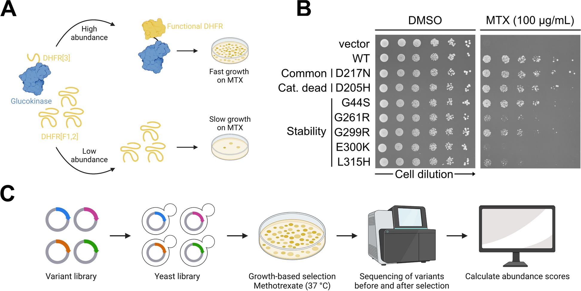
To assay for GCK variant abundance, the DHFR-PCA was used [31,32,33,34]. For plates, SC medium with leucine, methionine, and histidine was used. For selection, a final concentration of 100 \(\upmu\)g/mL methotrexate (Sigma-Aldrich, 100 mM stock in DMSO) and 1 mM sulfanilamide (Sigma-Aldrich, 1 M stock in acetone) were used. For control plates, a corresponding volume of DMSO was used. Plates were incubated for 4 days at 37 \(^\)C. As a vector control for DHFR-PCAs, pAG416GPD-EGFP-ccdB was used.

GCK activity assay

To assay for GCK activity, yeast cells were grown on SC medium without uracil containing 0.2 % D-glucose for 3 days at 30 \(^\)C.

Protein extraction

Yeast protein extraction was performed as described before [54]. Accordingly, 1.5–3 OD\(_\text \) units of exponential yeast cells were harvested in Eppendorf tubes (17,000 g, 1 min, RT). Proteins were extracted by shaking cells with 100 \(\upmu\)L of 0.1 M NaOH (1400 rpm, 5 min, RT). Then, cells were spun down (17,000 g, 1 min, RT), the supernatant was removed, and pellets were dissolved in 100 \(\upmu\)L 1.5× SDS sample buffer (1400 rpm, 5 min, RT). Samples were boiled for 5 min prior to SDS-PAGE.

Electrophoresis and blotting

To examine GCK protein levels, proteins in yeast extracts were separated by size on 12.5% acrylamide gels by SDS-PAGE. Subsequently, proteins were transferred to 0.2 \(\upmu\)m nitrocellulose membranes. Following western blotting, membranes were blocked in 5% fat-free milk powder, 5 mM NaN\(_3\), and 0.1% Tween-20 in PBS. Then, membranes were incubated overnight at 4 \(^\)C with a primary antibody diluted 1:1000. Membranes were washed 3 times 10 min with Wash buffer prior to and following a 1-h incubation with a peroxidase-conjugated secondary antibody. For detection, membranes were incubated for 2–3 min with ECL detection reagent (Amersham GE Healthcare) and were then developed using a ChemiDoc MP Imaging System (Bio-Rad). The primary antibody was anti-GFP (Chromotek, 3H9 3h9-100). The secondary antibody was HRP-anti-rat (Invitrogen, 31470).

Western blot quantification

To quantify protein levels from western blots, the Image Lab Software (Bio-Rad) was used. The software was used to measure the background-adjusted intensity of protein bands and the intensity of the Ponceau stain in the same lane. Then, a loading normalization factor was calculated for all lanes by dividing the ponceau intensity of lane 1 with that of all other lanes. Band intensities were adjusted by multiplying with their corresponding loading normalization factor. Finally, the loading-adjusted variant intensities were divided by the wild-type GCK intensity to obtain a normalized intensity that could be compared between replicates.

Glucokinase libraryCloning

Three regional pENTR221 libraries spanning aa 2–171 (region 1), 172–337 (region 3), and 338–465 (region 3) of the GCK sequence were previously generated [22]. To clone the entry libraries into the DHFR-PCA destination vector, each regional entry library was used for a large-scale Gateway LR reaction consisting of: 169.6 ng pENTR221-GCK library, 450 ng pDEST-DHFR-PCA vector, 6 \(\upmu\)L Gateway LR Clonase II enzyme mix (ThermoFisher), TE buffer to 30 \(\upmu\)L. The LR reactions were incubated overnight (RT). The following day, each reaction was terminated by incubation with 3 \(\upmu\)L proteinase K (37 \(^\)C, 10 min). For each region, 4 \(\upmu\)L LR reaction was transformed into 100 \(\upmu\)L NEB 10-beta electrocompetent E. coli cells. Following electroporation, cells were recovered in NEB 10-beta outgrowth medium (37 \(^\)C, 1 h). Then, cells were plated on LB medium with ampicillin and incubated overnight at 37 \(^\)C. If at least 500,000 colonies were obtained, cells were scraped from plates using sterile water. Plasmid DNA was extracted from cells corresponding to 400 OD\(_\text \) units (Nucleobond Xtra Midiprep Kit, Macherey-Nagel).

Yeast transformation

To express the GCK variant libraries in yeast, each regional plasmid library was transformed into the BY4741 yeast strain as described before [55] using the 30× scale-up. Briefly, yeast cells were grown overnight at 30 \(^\)C until late exponential phase. Cultures were then diluted with 30 \(^\)C YPD medium to an OD\(_\text \) of 0.3 in a minimum volume of 150 mL and were incubated with shaking for 4–5 h until two divisions had occurred. Then, cells were harvested and washed two times in sterile water (1200 g, 5 min, RT). The cell pellet was resuspended in a transformation mix consisting of 7.2 mL 50% PEG, 1.08 mL 1.0 M LiAc, 300 \(\upmu\)L 10 mg/mL single-stranded carrier DNA, 30 \(\upmu\)g plasmid library, and sterile water to 10.8 mL. The cell suspension was incubated in a 42 \(^\)C water bath for 40 min with mixing by inversion every 5 min. Cells were harvested (3000 g, 5 min, RT), the supernatant was removed, and cells were resuspended in 30 mL sterile water. To assess the transformation efficiency, 5 \(\upmu\)L cells were plated in duplicate on SC-uracil medium. The remaining cells were diluted in SC-uracil medium to an OD\(_\text \) of 0.2, and the cultures were incubated at 30 \(^\)C with shaking for 2 days until saturation.

If a minimum of 500,000 transformants were obtained, two cell pellets of 9 OD\(_\text \) units were harvested (17,000 g, 1 min, RT) and stored at −20 \(^\)C prior to DNA extraction to serve as technical replicates of the pre-selection condition.

In parallel to the library transformations, pEXP-DHFR-PCA wild-type GCK was transformed into the BY4741 yeast strain using the small-scale transformation protocol [53].

Selection

To select for GCK variant abundance, the yeast libraries were grown in duplicate on medium containing 100 \(\upmu\)g/mL methotrexate and 1 mM sulfanilamide. For each regional yeast library, 20 OD\(_\text \) units of cells were harvested in duplicate and were washed three times with sterile water (1200 g, 5 min, RT). The cells were resuspended in 500 \(\upmu\)L sterile water and each replicate was plated on a BioAssay dish (245 mm × 245 mm) containing SC+leucine+methionine+histidine medium with 100 \(\upmu\)g/mL methotrexate (Sigma-Aldrich) and 1 mM sulfanilamide (Sigma-Aldrich). The plates were incubated for 4 days at 37 \(^\)C. Following incubation, cells were scraped off each plate using 30 mL sterile water. Cell pellets of 9 OD\(_\text \) units were harvested (17,000 g, 1 min, RT) and stored at − 20 \(^\)C prior to DNA extraction.

In parallel, yeast cells expressing pEXP-DHFR-PCA wild-type GCK were also used for selection as described above but using 2.6 OD\(_\text \) units of yeast cells for each replicate, which were plated on petri dishes.

Plasmid DNA was extracted from yeast cells for two replicates pre- and post-selection, both for regional libraries and a wild-type GCK control. To extract plasmid DNA, the ChargeSwitch Plasmid Yeast Mini Kit (Invitrogen) was used.

Sequencing

In order to calculate the change in frequency of variants following selection, we sequenced the GCK ORF in plasmids extracted pre- and post-selection. Sequencing was done in 14 tiles spanning the GCK ORF, such that each regional library was covered by 4 or 5 tiles: region 1 (tiles 1–5), region 2 (tiles 6–10), and region 3 (tiles 10–14). The short tiles enabled sequencing of both strands in each tile to reduce base-calling errors. Although a limitation of using direct sequencing as a read-out is the risk of introducing PCR errors, the tileseqMave package (https://github.com/jweile/tileseqMave) used for data analysis accounts for the potential errors in multiple ways. First, amplicons derived from a wild-type GCK template were sequenced along with the non-selective and selective conditions, and variant frequencies observed in the wild-type control were subtracted from those observed in the non-selective and selective conditions. Second, the package performs quality filtering based on disagreement between the two replicates and variant counts in the non-selective condition.

First, the plasmid DNA extracted from yeast cells was adjusted to equal concentrations and was used for a PCR to amplify each tile. Each PCR consisted of 20 \(\upmu\)L Phusion High-Fidelity PCR Master Mix with HF Buffer (NEB), 1 \(\upmu\)L 10 \(\upmu\)M forward primer, 1 \(\upmu\)L 10 \(\upmu\)M reverse primer, 18 \(\upmu\)L plasmid library template. The following PCR program was used: 98 \(^\)C 30 s, 21 cycles of 98 \(^\)C 10 s, 63 \(^\)C 30 s, 72 \(^\)C 60 s, followed by 72 \(^\)C 7 min and 4 \(^\)C hold. Primer sequences can be found in the supplementary data (SKG_tilenumber_fw/rev).

Following tile amplification, Illumina index adapters were added to allow for multiplexing. For each indexing PCR, the following was mixed: 20 \(\upmu\)L Phusion High-Fidelity PCR Master Mix with HF Buffer (NEB), 2 \(\upmu\)L 10 \(\upmu\)M i5 indexing adapter, 2 \(\upmu\)L 10 \(\upmu\)M i7 indexing adapter, 1 \(\upmu\)L 1:10 diluted PCR product, 15 \(\upmu\)L nuclease-free water. The following PCR program was used: 98 \(^\)C 30 s, 7 cycles of 98 \(^\)C 15 s, 65 \(^\)C 30 s, 72 \(^\)C 120 s, followed by 72 \(^\)C 7 min and hold at 4 \(^\)C.

Following the indexing PCR, the indexed DNA fragments were pooled using equal volumes, and 100 \(\upmu\)L were run on a 4% E-gel EX Agarose Gel (Invitrogen) prior to gel extraction. Then, the quality and fragment size of the extracted DNA were examined using a 2100 Bioanalyzer system (Agilent), and the DNA concentration was adjusted using Qubit (ThermoFisher), before paired-end sequencing of the libraries using an Illumina NextSeq 550.

Data analysis

The TileSeqMave (https://github.com/jweile/tileseqMave, version 1.1.0) and TileSeq mutation count (https://github.com/RyogaLi/tileseq_mutcount, version 0.5.9) pipelines were used to calculate variant abundance scores from sequencing data.

Error calculation

Standard errors of abundance scores were calculated and refined using TileSeqMave (https://github.com/jweile/tileseqMave, version 1.1.0). In this pipeline, Bayesian refinement or regularization [56] is used to obtain more robust estimates of the standard errors. Briefly, linear regression of the fitness score and read counts from the pre-selection condition are used to obtain the prior estimate of the standard error. The empirical standard error is combined with the prior using Baldi and Long’s original formula, where \(\sigma _0\) represents the prior estimate of the standard error, \(v_0\) is the degrees of freedom given to the prior estimate, n represents the number of experimental replicates, and s is the empirical standard error:

$$\begin \sigma ^2 = \frac = \frac \end$$

Computational analysesDefining low-abundance threshold

To set a threshold for the abundance scores, we fitted the abundance score distribution using three Gaussians. These Gaussians represent the score distributions of variants with an abundance score comparable to nonsense variants, intermediate variants, and synonymous variants, respectively. To define a cutoff for variants with decreased abundance, we used the intersection of the second and last Gaussian.

Structure modeling and visualization

Protein structures were visualized and rendered using UCSF ChimeraX (v1.4), developed by the Resource for Biocomputing, Visualization, and Informatics at the University of California, San Francisco [57, 58]. The region spanning residues 157–179 missing from the crystal structure of the GCK super-open conformation (PDB: 1V4T) is shown in dashed lines in Fig. 4, but was modeled using Modeller [59] to be able to obtain \(\Delta \Delta G\) estimates for variants in the region. Five structural models were generated with the Model Loops interface for Modeller available in ChimeraX (v1.3) using the super-open GCK structure (PDB: 1V4T) and the canonical GCK sequence (UniProt: P35557-1) as inputs. HETATM records and non-native terminal residues were removed from the PDB file using pdb-tools v2.4.3 [60] prior to the loop structure generation. Model Loops was run using the standard protocol, modeling only internally missing structure, and without allowing for any remodeling of residues adjacent to the missing segment.

Calculation of thermodynamic stability changes

Changes in protein thermodynamic stability (\(\Delta \Delta G\) = \(\Delta G_\text - \Delta G_\text \)) caused by single-residue substitutions were predicted with Rosetta (GitHub sha1 c7009b3115 c22daa9efe2805d9d1ebba08-426a54) using the Cartesian ddG protocol [44]. Structure preparation and relaxation and the following \(\Delta \Delta G\) calculations were performed using an in-house pipeline (https://github.com/KULL-Centre/PRISM/tree/main/software/rosetta_ddG_pipeline, v0.2.1). Rosetta \(\Delta \Delta G\) output values were divided by 2.9 to convert from Rosetta energy units to kcal/mol [41, 44]. \(\Delta \Delta G\) predictions for all possible point mutations in the segment spanning residues 157–179 were calculated for the super-open conformation of GCK based on the structural models created as described above. Predictions were performed for each of the five different structural models individually and subsequently averaged. For all analyses using \(\Delta \Delta G\) predictions in this study, the values for the 157–179 region in the super-open conformation were used to supplement our previously reported \(\Delta \Delta G\) values [22].

We performed additional \(\Delta \Delta G\) calculations for this work using as input the structure of the closed GCK conformation bound to the glucose substrate, with glucose kept in the position observed in the crystal structure (PDB: 1V4S). \(\Delta \Delta G\) value changes associated with the presence of the ligand were analyzed by comparing the results to our previous \(\Delta \Delta G\) calculations, which were based on the closed conformation without substrate bound [22]. For the analysis, glucose binding site residues were defined as residues positioned less than 4 Å away from glucose, with the distance between each protein residue and glucose defined as the shortest distance between any heavy atom in glucose and the residue. Variants were defined as decreasing substrate binding affinity when the calculated variant \(\Delta \Delta G\) was at least 2 kcal/mol larger in the glucose-bound structure than in the glucose-free structure.

Calculation of solvent accessible surface area and weighted contact number

The absolute solvent accessible surface area of every residue in both the closed (PDB: 1V4S) and super-open (PDB: 1V4T, with residues 157–179 added as described under the “Structure modeling and visualization” section) crystal structure conformations of GCK was calculated using DSSP [61] and normalized to a relative value (rASA) using a theoretically derived maximum accessibility per residue [62]. Residues with rASA \(\le\) 0.2 were categorized as structurally buried, while residues with rASA > 0.2 were categorized as solvent-exposed. Moreover, a weighted contact number (WCN) was calculated for every residue i in the structures using the expression

$$\begin \text _ = \sum \limits _ s(r_) \text s(r)=\frac\right) ^6}\right) ^}, \end$$

(1)

where \(r_\) is the distance between residues i and j, and \(r_0\) = 7 Å. Interresidue distances were evaluated using the MDTraj (v1.9.7, [63]) function compute_contacts. Distances were measured as the shortest distance between any interresidue pair of atoms for residue pairs involving glycine and as the shortest distance between any two sidechain heavy atoms for all other residue pairs.

Molecular dynamics simulationsPreparation of starting structures

We performed atomistic molecular dynamics simulations of wild-type GCK and five GCK single substitution variants (D158A, G162Q, A173F, G175E, V455M) starting from both closed and super-open conformations of each variant. The simulation starting structures were prepared using the closed conformation crystal structure (PDB: 1V4S) and the super-open conformation crystal structure (PDB: 1V4T) with residues 157–179 added to the structure using Modeller [59], as described under the “Structure modeling and visualization” section. Mutations were introduced to the structures using the PyMOL (v2.5.2) Mutagenesis Wizard [64] by always selecting the mutant side chain rotamer with the smallest structural “strain.” In all structures, terminal charges were neutralized by capping with an acetyl group in the N-terminus and an amino group in the C-terminus, and non-native N-terminal residues present in the crystal structures were mutated to match the canonical GCK sequence (UniProt: P35557-1).

Simulation setup

All simulations were performed with Gromacs (v2021.1) [65] using the a99SB-disp force field in combination with the a99SBdisp water model [66]. Each system was prepared by placing the protein structure in the center of a dodecahedral box at least 1.1 nm from the box boundary. The protonation states of functional groups were set to match a pH value of 7.4 after evaluating the effective pKa values of all groups using ProPKA [67, 68]. The protonation site in singly protonated histidine residues was assigned automatically by Gromacs. After solvation with water molecules, counter ions were added to neutralize the system and additional ions (Na\(^+\) and Cl\(^-\)) were added to reach an ion concentration of 0.15 M. Na\(^+\) ions originally present in the crystal structures were kept.

System preparation was followed by energy minimization by steepest descent with an initial minimization step size of 0.01 nm and until the maximum system force was smaller than 1000 kJ mol\(^\) nm\(^\). A four-step equilibration protocol was then applied to make sure that all protein structures were stable in the simulations. First, the thermostat target temperature was linearly increased from 10 to 200 K during a 5-ns NVT simulation in which position restraints with a force constant of 1000 kJ mol\(^\) nm\(^\) were applied to all protein heavy atoms. Second, the target temperature was further linearly increased from 200 to 310 K during another 5-ns NVT simulation with position restraints only on the protein C\(\alpha\) atoms. Third, all position restraints were dropped, and pressure was equilibrated to 1 bar using the Berendsen barostat [69] in a 3-ns NPT simulation. Fourth, equilibration was finalized by switching to the Parrinello-Rahman barostat [70] and extending the simulation time with 3 ns. Following equilibration, production simulations were run for 1 µs at 310 K and 1 bar, saving the system conformation every 100 ps. All simulations were run in replicas of three (different random velocities were used to initialize each replica) producing three trajectories for every GCK variant in each GCK starting conformation.

In all simulations, covalent bonds involving hydrogen atoms were constrained with the LINCS algorithm [71]. Van der Waals interactions and short-range electrostatic interactions were evaluated with a 1.2-nm cutoff [66]. For van der Waals interactions, the force was shifted and smoothly switched to zero between 1 and 1.2 nm. The neighbor list was updated at least every 10th step. Long-range electrostatic interactions were calculated with the smooth particle mesh Ewald method [72] with a grid spacing of 0.16 nm and an interpolation order of four. The leap-frog algorithm was used for integration with a timestep of 2 fs. For both equilibration and production, temperature was controlled with the velocity-rescaling thermostat [73], treating protein and non-protein atoms as separate coupling groups, and with a coupling time constant of 1 ps. Pressure coupling was applied with a time constant of 2 ps and setting compressibility to 4.5\(\cdot 10^\) bar\(^\) for both the Berendsen and Parrinello-Rahman barostats.

Trajectory analysis

Production trajectories were analyzed with Gromacs (v2021.1) [65] and MDTraj (v1.9.7) [63]. Raw trajectory files were processed with the Gromacs tool trjconv to center the protein in the simulation box and to remove non-protein species prior to further analysis. MDTraj was used to calculate the backbone heavy atom RMSD between all simulated structures and the wild-type GCK crystal structures. The RMSD calculations were carried out separately for each protein domain, with domain definitions used for the simulation analysis specified in Additional file 2. RMSF values were similarly evaluated for each domain with MDTraj from the fluctuations of C\(\) atoms around the average simulation structures. Angles and distances between atoms were also calculated with MDTraj tools. The cleft angle between the small and large domains of GCK was monitored by calculating the angle between the C\(\) atoms of residues 109, 233, and 229, while the movement of helix 13 was studied by calculating the distance between the C\(\) atoms of residues 159 and 452. The cleft angle definition was inspired by previous work in which the 159–452 distance was also introduced and monitored [30].