The remainder of this work focuses on proving Theorem 2.1. As such, from now on we only consider the fixed sequence \(\Lambda _N^:=\Lambda _N^(})\) defined as in (2.1). We emphasize once again that all vertices \(v\in \Lambda _N^\) satisfy \(\deg (v)\in \\), and in particular, all boundary vertices have degree three, and two of their edges are contained in \(\Lambda _N^\). To further simplify notation, set

$$\begin \mathfrak _N^: = \mathfrak _}, \quad H_N^: = H_}, \quad _N^}:= _}, \quad \mathring}_N^}:= __N^}. \end$$

(4.1)

Since we will frequently consider subgraphs of both \(\Gamma ^\) and \(\Lambda _N^\), we denote their respective sets of vertices and bonds by

$$\begin \Gamma ^ \equiv (^, ^), \quad \Lambda _N^ \equiv (_N^, _N^). \end$$

(4.2)

There are two goals of this section. The first is to give a nice description for the ground state space of \(H_N^\). This is achieved in Sect. 4.1 by considering the Weyl representation of \(\mathfrak (2)\) acting on a Hilbert space of homogeneous polynomials. Each ground state can be uniquely described by a polynomial supported on the boundary \(\partial \Lambda _N^\). As we are interested in calculating the ground state expectation of observables supported sufficiently far away from this boundary, a finite volume “bulk-boundary map” will be identified that can be used to calculate the expected value of any such observable in the ground state associated with any fixed boundary polynomial. A “bulk state” will also be defined which will be used to prove Theorem 2.1 in Sect. 5. This will be done by showing that the bulk state well approximates each of the finite volume ground states and, moreover, converges strongly to the unique infinite volume ground state. The second goal of this section is to rewrite these maps in terms of hard-core polymer representations. The graphs and weights used for this representation are introduced in Sect. 4.2, and the final expressions are proved in Sect. 4.3. A lemma producing an initial comparison between the bulk-boundary map and the bulk state is then proved in Sect. 4.5, from which we will obtain the indistinguishability bound in Sect. 5.

4.1 The Ground States and Bulk State of the Decorated AKLT Hamiltonian

We follow the construction in [35] and use the Weyl representation of the Lie algebra \(\mathfrak (2)\) acting on polynomials in two variables to explicitly realize the AKLT mode on the decorated lattice. For the convenience of the reader, we review the relevant setup and ground state description from this work. As such, consider the Hilbert space of complex homogeneous polynomials of degree m

$$\begin \begin \mathcal ^:= \left\^ \lambda _ u^k v^ \,: \, \lambda _k\in \right\} \subset \mathbb [u,v], \end \end$$

(4.3)

where the inner product is taken so that the monomial basis is orthogonal. Concretely, using the change of variables

$$\begin u= \exp (i \phi /2)\cos (\theta /2), \quad v=\exp (-i\phi /2) \sin (\theta /2), \end$$

(4.4)

and given any pair \(\Phi ,\Psi \in \mathcal ^\), the inner product is

$$\begin \langle \Phi , \Psi \rangle&= \int d\Omega ~ \overline \Psi (\theta ,\phi ) \end$$

(4.5)

$$\begin d\Omega = \frac \sin&(\theta ) d\phi d\theta , \;\; 0 \le \phi< 2\pi , \; 0\le \theta < \pi . \end$$

(4.6)

In particular, this allows one to view each \(\mathcal ^\) as a subspace of \(L^2(d\Omega ).\)

The on-site Hilbert space for the decorated AKLT model is then \(\mathfrak _x = \mathcal ^\) for each vertex \(x\in \Gamma ^\). Thus, \(\mathfrak _\Lambda = \bigotimes _\mathcal ^\) for any finite \(\Lambda \subseteq \Gamma ^\), and the associated inner product is

$$\begin \langle \Phi , \Psi \rangle&= \int d\varvec^ ~ \overline)} \Psi (\mathbf ) , \quad \forall \, \Phi ,\Psi \in \mathfrak _\Lambda \,. \end$$

(4.7)

In the above, \(d\varvec^\) is the product measure associated with \(\\) and \(\Phi (\mathbf )\) denotes the function resulting from appropriately applying the change of variables (4.4) independently to each pair of variables \(u_x,v_x\) associated with any \(x\in \Lambda \). For simplicity, we denote by \(\theta = (\theta _x)_\), and \(\phi =(\phi _x)_\).

The local AKLT Hamiltonian from (2.2) is represented on \(\mathfrak _\Lambda \) using the Weyl representation. For each \(m\ge 0\), this is the irreducible representation \(\pi _m: \mathfrak (2)\rightarrow B(\mathcal ^)\) given by

$$\begin \begin \pi _m(\sigma ^3) = v\partial _v - u\partial _u, \hspace \pi _m(\sigma ^-) = u\partial _v,\hspace \pi _m(\sigma ^+) = v\partial _u, \end \end$$

(4.8)

where \(\sigma ^3\) is the third Pauli matrix, and \(\sigma ^\) are the usual lowering and raising operators. This is isomorphic to the spin-m/2 representation. For adjacent sites x and y, with degrees \(m_x\) and \(m_y\), respectively, the subspace of \(\mathfrak _x \otimes \mathfrak _y\) corresponding to the maximal spin \((m_x + m_y)/2\) is spanned by the states \((u_x\partial _ + u_y\partial _)^kv_x^v_y^\) where \(0 \le k \le m_x+m_y\), as one can check by evaluating these states against the tensor product representation \(\pi _\otimes \pi _\) of \(\mathfrak (2)\). The orthogonal projection onto this subspace then gives the AKLT interaction term \(P_\in B(\mathfrak _x \otimes \mathfrak _y)\). In this representation, the ground state space \(\ker \) is characterized by boundary polynomials. Indeed, by a simple argument from [35],

$$\begin \begin \ker } = \left\_x \otimes \mathfrak _y: f = (v_xu_y - u_xv_y) g(u_x,v_x, u_y,v_y) \right\} , \end \end$$

(4.9)

where g is a homogeneous polynomial of degree \(\deg (x)-1\) in \(u_x\) and \(v_x\), and similarly in the y-variables. In a word, the ground state requires that there be a singlet \(v_xu_y-u_xv_y\) across the bond (x, y), but the remaining variables can form any homogeneous polynomial of the appropriate degree. By the frustration-free property, a ground state of any finite volume Hamiltonian \(H_\Lambda \) must project all edges \((x,y)\in \Lambda \) into a singlet. Since \(}_x = ^\) and the polynomials over \(\mathbb \) form a unique factorization domain, (4.9) immediately implies the following description for the ground state space.

Theorem 4.1

[35, 36]. Let \(d\ge 0\). For any finite \(\Lambda \subseteq \Gamma ^\), the ground state space is given by

$$\begin \ker (H_\Lambda ) = \left\(u_iv_j-v_iu_j)\in \mathfrak _\Lambda : g\in }_^}\right\} \end$$

(4.10)

where the set of all possible boundary polynomials is

$$\begin }_^\textrm=\bigotimes _ ^, \quad d_i = \deg (i)-\deg _\Lambda (i). \end$$

(4.11)

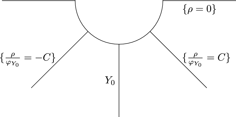
Note that \(d_i\) is the number of edges connected to i that are not contained in \(\Lambda \). In the case of \(\Lambda _N^\), since \(d_i=1\) for all \(i\in \partial \Lambda _N^\), see Fig. 2, the space of boundary polynomials, \(}_}^}\), is spanned by all elements of the form

$$\begin\prod _}\left( a_iu_i+(1-a_i)v_i\right) , \quad a_i\in \.\end$$

Therefore, \(\dim ( \ker H_N^) = 2^|}=2^\) by Proposition 6.2.

The matrix entries of an operator \(A \in _N^\) can be conveniently described using the change of variables (4.4) by introducing the symbol of A, denoted \(A(\varvec)\). Let

$$\begin \Omega _x=(\sin \cos ,\sin \sin ,\cos ) \end$$

(4.12)

be spherical coordinate associated with \(x\in \Lambda _N^\). Arovas, Auerbach and Haldane showed in [4] that

$$\begin \langle \eta , A \xi \rangle = \int d\varvec^} ~\overline \xi (\theta ,\phi ) A(\varvec), \quad \forall \eta , \xi \in \mathfrak _N^, \end$$

(4.13)

where \(A(\varvec)\) is a continuous function of the angles \(\theta _x,\phi _x\) associated with \(x\in \text (A)\).

In general, the symbol is not unique. However, a specific choice can be made by first defining it unambiguously for a basis of the on-site algebra \(B(^)\) and invoking linearity to define the symbol for a general \(A\in B(^)\). We require \(\mathbb (\Omega )=1\) so that the support condition stated after (4.13) is satisfied. This is achieved by including \(\mathbb = 1\) in the on-site basis and implementing the following procedure. First, use the commutation relation \([\partial _x, x]=1\) to rewrite each basis element as

$$\begin A = \sum __0}\sum _ a_ \partial _u^k \partial _v^l u^v^, \quad a_\in . \end$$

Then, using \(\langle , v^\Psi }\rangle =C_\langle , v^\Psi }\rangle \) where \(C_ = \frac\), define the symbol to be

$$\begin A(\Omega ):=\sum __0}\sum _ C_a_ \overline u^v^, \end$$

(4.14)

which is to be understood using (4.4). The formula extends to any \(A\in _}^}\) in the usual way: \(\left( \bigotimes _A_x\right) (\varvec):= \prod _x A_x(\Omega _x)\) for a product of on-site observables, and then extended to any local operator by linearity. The convention \(\mathbb (\Omega )=1\) implies \(AB(\varvec) = A(\varvec)B(\varvec)\) if A, B have disjoint support.

The matrix elements formula (4.13) can also be used to calculate ground state expectations for any \(\Psi (f)\in \ker H_N^\) with boundary polynomial \(f\in }_}^}\) as

$$\begin \langle , \rangle = \int d\varvec^}\prod _}|u_i v_j - v_i u_j|^2 |f|^2A(\varvec). \end$$

(4.15)

The change of variables (4.4) can also be used to show \(|u_i v_j - v_i u_j|^2 = \frac (1- \Omega _i \cdot \Omega _j).\) Thus, setting

$$\begin d\rho _^}=\rho _^} d\varvec^^}, \quad \rho _} = 2^_N^|}\prod _^} (1-\Omega _i \cdot \Omega _j), \end$$

(4.16)

the ground state expectation \(\langle , \rangle \) can then be rewritten in terms of \(|f|^2\) and a bulk-boundary map \(\mathring_(A;\partial \varvec)\) that is independent of \(f\in }_}^}\) as follows.

Lemma 4.2

(Bulk-boundary map). Fix \(N\ge 2\) and let \(\Psi (f)\in \ker H_^\) be a nonzero ground state associated with a boundary polynomial \(f\in }_}^}\) as in Theorem 4.1. Then, for any \(K<N\),

$$\begin \langle , \rangle = \int d\rho _^}\, |f|^2\, \mathring_N(A;\partial \varvec), \quad A\in _K^ \end$$

(4.17)

where \(\mathring_N(A;\partial \varvec):=\mathring_(A;\partial \varvec)/\mathring_N(\partial \varvec)\) is the function of the boundary variables \(\partial \varvec= ( \Omega _x: x\in \partial \Lambda _N^)\) defined by

$$\begin \mathring_(A;\partial \varvec):= \int d\varvec^_^} \rho _^} A(\varvec), \quad \mathring_N(\partial \varvec):=\mathring_N(\mathbb ;\partial \varvec). \end$$

(4.18)

Proof

We first show that \(\mathring_N(A;\partial \varvec)\) is well defined on all sets with positive measure. For any fixed choice of the boundary variables \(\partial \varvec\), the map \(A \mapsto \mathring_N(A;\partial \varvec)\) is a ground state of \(H__N^}\). To see this, fix the values of \(v_i(\theta _i,\phi _i),u_i(\theta _i,\phi _i)\) for each \(i\in \partial \Lambda _N^\), and consider the function \(g_}\) defined by

$$\begin g_} = \prod _ (i,j)\in \Lambda _N^: \\ i\in \partial \Lambda _N^ \end}(u_iv_j-v_iu_j)\in }__N^}^}. \end$$

(4.19)

In the above, we observe that any site \(j\in \Lambda _N^\) that neighbors \(i\in \partial \Lambda _N^\) is necessarily an interior site for all \(N\ge 2\), and so, \(g_}\) is nonzero. By Theorem 4.1, \(\Psi (g_})\in \ker (H__N^})\), and as a consequence, \(\mathring_N(A;\partial \varvec) = \langle })}, })}\rangle \). This implies that \(\mathring_N(\mathbb ) = \left\| \Psi (g_}) \right\| ^2 \ne 0\), and \(\mathring_N(A; \partial \varvec)\) is a bounded, continuous function of the boundary variables for each A. Hence, (4.18) is well defined, and so too is \(\mathring_N(A;\partial \varvec)\). As a consequence, (4.17) follows immediately from the matrix element formula (4.15) since

$$\begin \langle \Psi (f), A \Psi (f) \rangle&= \int d\varvec^}} |f|^2 \rho _} A(\varvec) \\&= \int d\varvec^}} |f|^2 \int d\varvec^_N^} ~ \rho _} \left[ \frac^_N^}\rho _} A(\varvec) }^_N^} ~ \rho _}} \right] . \end$$

\(\square \)

We now introduce the bulk state, \(\omega _N(A)\), which we show well approximates \(\langle , \rangle \) as in (4.17) when \(K<<N\). This is motivated from averaging the bulk-boundary function \(\mathring_N(A;\partial \varvec)\) over the possible values of the boundary variables. Explicitly, \(\omega _N(A):= Z_N(A)/Z_N\) where

$$\begin Z_N(A) := \int d\rho _^}~ A(\varvec), \quad A\in _N^ \end$$

(4.20)

and \(Z_N:= Z_N(\mathbb )\). Note that, if \(A \in _K^\) with \(K<N\) one has that, indeed,

$$\begin Z_N(A) = \int d\varvec^} \mathring_N(A;\partial \varvec). \end$$

It is not immediately obvious from (4.20) if \(\omega _N\) is a ground state for \(H_^\), or even if it is positive on all of \(_N^\). However, it is a ground state of \(H_K^\) for all \(K<N\). To see this, let us consider the AKLT model obtained by replacing the spin-3/2 at all boundary sites \(x\in \partial \Lambda _N^\) with a spin-1, where the nearest-neighbor interaction is still defined as the orthogonal projection onto the largest spin subspace between any pair of adjacent sites. The natural variation of Theorem 4.1 applies in this case, yielding a unique ground state given by \(\Psi _N = \prod _}(u_iv_j-v_iu_j)\). We observe that, for \(A \in _K^\) with \(K<N\),

$$\begin Z_N(A) = \langle , \rangle , \quad \quad Z_N = \left\| \Psi _N \right\| ^2. \end$$

As this modified model does not change the spin or interaction terms for sites of \(\Lambda _K^\), \(\omega _N\) is then a ground state of \(H_K^\) by frustration-freeness.

Notice that for any normalized \(\Psi (f)\in \ker H_N^\) and observable \(A\in _K^\) with \(K<N\) one

$$\begin | \langle \Psi (f), A \Psi (f) \rangle - \omega _(A) | = \left| \int d\rho _^} \,|f|^2 \, \left[ \mathring_N(A;\partial \varvec)-\omega _N(A) \right] \right| ,\nonumber \\ \end$$

(4.21)

where we have used that \(\int d\rho _^}} \,|f|^2 =\Vert \Psi (f)\Vert ^2=1 \). The ground state indistinguishability result, Theorem 2.1, will then be a consequence of producing an upper bound on the rate at which \(\sup _}|\mathring_N(A;\partial \varvec)-\omega _N(A)|\rightarrow 0\) as \(N\rightarrow \infty \). This will be achieved using a cluster expansion associated with a hard-core polymer description of \(\omega _N(A)\) and \(\mathring_N(A;\partial \varvec)\), the latter of which we now discuss.

4.2 Graphs and Weights for the Hard-Core Polymer Representation

To bound the right-hand side of (4.21), the maps \(Z_N(A)\) and \(\mathring_N(A;\partial \varvec)\) will be rewritten in terms of a set of polymers and weight functions. The sets used for each map will be slightly different, and so, we introduce these in a rather general setting. We begin by establishing some basic graph notation and conventions.

Definition 4.3

Two connected subgraphs G and H of \(\Gamma ^\) will be called (pairwise) connected, denoted if \(G \cup H\) is a connected graph. Otherwise, G and H are not connected, and we write G|H. More generally, if \(\\) and \(\\) are the connected components of graphs G and H, respectively, we say G and H are not connected, denoted G|H, if \(G_i|H_j\) for all i and j. Otherwise, G and H are connected and we write .

Note that if G and H are connected subgraphs of \(\Gamma ^\) then G|H if and only if \(_G\cap _H= \emptyset \).

Definition 4.4

A collection of connected graphs \(\\) is said to be hard core if they are pairwise not connected, i.e., \(G_k|G_l\) for all \(k\ne l\).

We are now ready to introduce the set of polymers of interest. The particular subgraphs of interest are connected graphs \(\phi \subseteq \Gamma ^\) such that \(1\le \deg _\phi (v)\le 2\) for all \(v\in \phi \). Such graphs will be called self-avoiding and are partitioned into the set of closed loops \(^\), and the set of self-avoiding walks \(^\):

$$\begin ^&: = \ \text : \deg _\phi (v) = 2 \; \forall \, v\in _\phi \} \end$$

(4.22)

$$\begin ^&:= \ \text : 1\le \deg _\phi (v) \le 2 \; \forall \, v\in _\phi \} ^. \end$$

(4.23)

Each self-avoiding walk \(\phi \) has exactly two vertices \(\\) such that \(\deg _\phi (v)=\deg _\phi (w)=1\), called the endpoints, and all other vertices have degree two in G. For convenience, we will denote \(}(\phi )\) the set of endpoints of a self-avoiding walk \(\phi \).

The subset of self-avoiding walks of interest \(^\subsetneq ^\) are those whose endpoints belong to \(\Gamma ^\):

$$\begin ^:= \^: }(\phi ) \subset \Gamma ^ \}. \end$$

(4.24)

The set of all possible polymers is then given by

$$\begin ^:= ^\cup ^. \end$$

(4.25)

Since the endpoints of every walk from \(^\) belong to \(\Gamma ^\), the map

$$\begin \iota _d: ^ \rightarrow ^ \end$$

(4.26)

obtained from replacing the spin-1 chain between \((v,w)\in \Gamma ^\) by an edge is a bijection. As a convention, the “length” of a polymer is taken to be the number of edges in its undecorated representative:

Definition 4.5

For any undecorated polymer \(\phi \in \mathcal ^\), define the length to be the number of edges in \(\phi \), i.e., \(\ell (\phi ) = | _\phi |.\) For any decorated polymer \(\phi \in ^\), define the length by \(\ell (\phi ):= \ell (\iota _d(\phi ))\) where \(\iota _d\) is the bijection from (4.26).

Note that the total number of edges \(|_\phi |\) for any \(\phi \in ^\) is \((d+1)\ell (\phi )\). Since \(\Gamma ^\) is bipartite, any closed loop \(\phi \in ^\) necessarily has even length.

We will need to consider specific subsets of \(^\) in order to derive the polymer representation of \(Z_N(A)\) and \(\mathring_N(A; \partial \varvec)\). For the convenience of the reader, we introduce them now.

For \(0< K < N\), let \(_^\subseteq ^\) the set of closed loops in \(\Lambda _N^\) which do not intersect \(\Lambda _K^\):

$$\begin _^:= \^: \phi \subset \Lambda _N^,\, \phi |\Lambda _K^ \}, \end$$

(4.27)

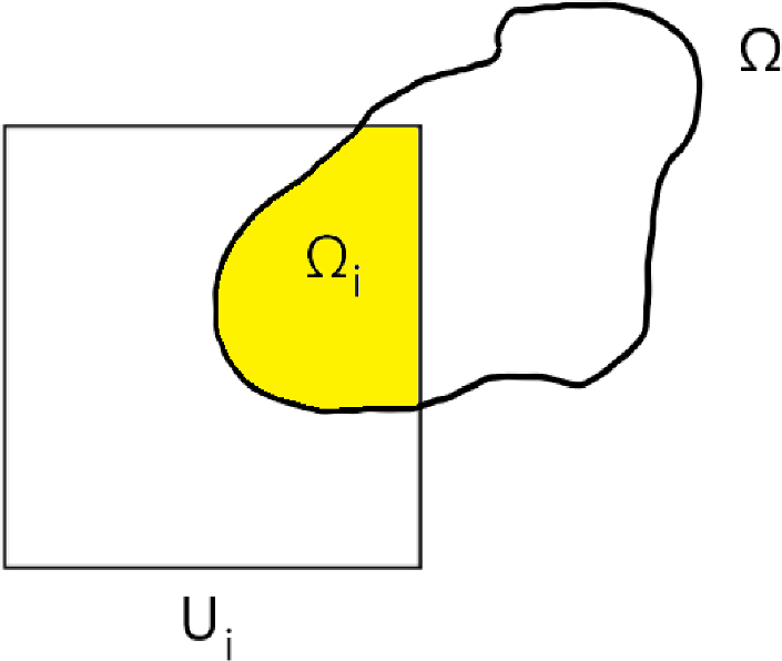
and \(_^:= \^: \phi \subset \Lambda _N^ \}\). Moreover, let \(\mathcal _^\subseteq ^\) be the set of self-avoiding walks with edges in \(\mathcal _N^ \mathcal _K^\) and endpoints in \(\Lambda _K^\) (see Fig. 4):

$$\begin \mathcal _^:= \^: \mathcal _\phi \subset \mathcal _N^ \mathcal _K^,\, }(\phi ) \subset \partial \Lambda _K^ \}. \end$$

(4.28)

Then we define, for \(K >0\),

$$\begin \mathcal _^&:= _^ \cup \mathcal _^ \end$$

(4.29)

and \(\mathcal _^ = \mathcal ^_\). This is the set of polymers we will use in the representation of \(Z_N(A)\). Note that \(\iota _d(_^)=_^\).

In the representation of \(\mathring_N(A;\partial \varvec)\), we will also have to consider self-avoiding walks that begin or end at \(x\in \partial \Lambda _N^\). Explicitly, for \(K>0\), we denote by

$$\begin \mathring}_^:= \^: \mathcal _\phi \subset \mathcal _N^ \mathcal _K^,\, }(\phi ) \subset \partial \Lambda _K^\cup \partial \Lambda _N^\} \end$$

(4.30)

the set of all self-avoiding walks with edges contained in \(_N^_K^\) and endpoints in \(\partial \Lambda _K^\cup \partial \Lambda _N^\). For the special case \(K=0\), we consider only the self-avoiding walks which begin and end at \(\partial \Lambda _N^\):

$$\begin \mathring}_^:= \^: \mathcal _\phi \subset \mathcal _N^ \mathcal _K^,\, }(\phi ) \subset \partial \Lambda _N^ \}. \end$$

(4.31)

Then similarly to before, we define for \(K \ge 0\)

$$\begin \mathring}_^:= _^ \cup \mathring}_^. \end$$

(4.32)

Now that we have introduced the polymer sets of interest, we turn to introducing a weight function \(W_d\) on \(^\) that will express how much a give polymer contributes to the polymer representation of \(Z_N(A)\) or \(\mathring_N(A;\partial \varvec)\).

The weight of any \(\phi \in ^\) is defined analogously to those given by Kennedy, Lieb and Tasaki in [35]. This is a consequence of evaluating certain integrals which naturally arise when calculating ground state expectations. For any closed loop \(\phi \in ^\), the weight \(W_d(\phi )\) is

$$\begin W_d(\phi ):= (1/3)^ = \int d \varvec^~ \prod _-\Omega _i \cdot \Omega _ j, \end$$

(4.33)

where \(\subset \Gamma ^\) is any finite subset of vertices such that \(\mathcal _\phi \subset \). Similarly, if \(\phi \in ^\) is a self-avoiding walk with endpoints \(v,w\in \Gamma ^\), the weight function \(W_d(\phi )\) is

$$\begin W_d(\phi ):= (-1/3)^\partial \phi (\varvec) = \int d \varvec^} ~ \prod _ -\Omega _i \cdot \Omega _ j \end$$

(4.34)

where \( \partial \phi (\varvec): = - \Omega _ \cdot \Omega _\) and \(\subset \Gamma ^\) is any finite set of vertices such that \(\mathcal _\phi \cap = \mathcal _\phi \left\ \).

In either case, (4.33) and (4.34) and their independence of the set \(\) are easy to verify by first integrating \(\int d \varvec^x = 1\) for all sites \(x\in \mathcal _\phi \), and using \(\deg _\phi (x)=2\) for every \(x\in \cap _\phi \) to evaluate

$$\begin\int d \varvec^\cap _\phi } \prod _ -\Omega _v \cdot \Omega _w = (-1)^\int d \varvec^\cap _\phi } \prod _ \Omega _v \cdot \Omega _w \end$$

by successively applying

$$\begin \int d \Omega _x(\Omega _y\cdot \Omega _x)(\Omega _x\cdot \Omega _z) = \frac\Omega _y\cdot \Omega _z. \end$$

(4.35)

The exponents in (4.33)–(4.34) count the number of vertices to which (4.35) is applied. In the case of the closed loop, integrating over the final site \(x\in \mathcal _\) yields \(\int d \Omega _x(\Omega _x\cdot \Omega _x) = 1\) as \(\Omega _x\) has unit length. The expression (4.35) can be explicitly computed using (4.6) and (4.12).

4.3 The Hard-Core Polymer Representation of \(Z_N\)

In [35], Kennedy, Lieb and Tasaki used a loop gas representation of the ground state with a hard-core condition to evaluate ground state expectations when \(d=0\). Their methods can also be used for the decorated models. Here we prove Lemma 4.6 which establishes a modified version of this representation for

$$\begin Z_N(A) = 2^_N^|} \int d\varvec^^}~ \prod _^} (1-\Omega _i \cdot \Omega _j) A(\varvec). \end$$

(4.36)

To rewrite \(Z_N(A)\), we follow [35] and distribute the product from (4.36) to find

$$\begin \prod _^} (1-\Omega _i \cdot \Omega _j) = \sum __N^} \prod _(-\Omega _i \cdot \Omega _j). \end$$

(4.37)

where \( _N^\) is the collection of all subgraphs of \(\Lambda _N^\) with no isolated vertices

$$\begin _N^:= \: \deg _G(v)> 0 \; \forall v\in G\}. \end$$

(4.38)

Inserting this into (4.36), the sum is then simplified by removing subgraphs for which

$$\begin \int d\varvec^^} \prod _(-\Omega _i \cdot \Omega _j) A(\varvec) = 0. \end$$

(4.39)

The graphs that remain are characterized by their connected components, which necessarily form a hard-core set.

The next result, which shows \(Z_N(A)\) can be written in terms of hard-core subsets of \(_^\), is a slight simplification of [35, Equation 4.14]. We follow their method of proof, which is a consequence of observing that the variable \(\Omega \) associated with a single site satisfies

$$\begin \int d \Omega ~ f(-\Omega ) = \int d\Omega ~ f(\Omega ). \end$$

(4.40)

As the integral is taken over \([0,\pi ]\times S^1\), this can easily be verified from recognizing that the measure \(d\Omega \) is invariant under the diffeomorphism \(R: [0, \pi ] \times S^1 \rightarrow [0,\pi ]\times S^1\) that sends \(\Omega \mapsto -\Omega \) defined by \(R(\theta ,\phi ) = (\pi - \theta , \phi + \pi )\) (Fig. 4).

Fig. 4

Example of polymers from \(_^\). The decoration is suppressed outside of \(\Lambda _2^\) for clarity

Lemma 4.6

Fix \(N>K\ge 0\) and \(d\ge 0\). Then for any \(A\in _K^\),

$$\begin Z_N(A) = \int d\rho _} A(\varvec) \Phi _(\varvec) \end$$

(4.41)

where with respect to the weight functions from (4.33)–(4.34),

$$\begin \Phi _(\varvec):= 2^_N^_K^|}\sum ^ _ \subseteq _^ } W_d(\phi _1)\cdots W_d(\phi _n), \end$$

(4.42)

and the notation indicates the sum is taken over all hard-core collections \(\left\ \subset _^\).

The sum appearing in the definition of \(\Phi _\) is finite, and moreover, each product \(W_d(\phi _1)\cdots W_d(\phi _n)\) is necessarily a (real-valued) monomial in the variables \(\Omega _\) associated with the boundary \(x\in \partial \Lambda _K^\). Also notice that \(Z_N = \int d\rho _^} \Phi _(\varvec)\).

Proof

Fix a subgraph \(G\in _N^\). If there is a \(x\in G \Lambda _K^\) such that \(\deg _G(x)\) is odd, then applying (4.40) to this vertex implies

$$\begin \int d\Omega _x \prod _(-\Omega _x \cdot \Omega _y) = 0. \end$$

(4.43)

As the symbol \(A(\varvec)\) is constant in the variables \(\Omega _v\) for all \(v\in \Lambda _N^\Lambda _K^\), by first integrating over this vertex x one sees that G satisfies (4.39) by (4.43). By definition of \(_^\), the degree of any vertex \(x\in G\) is at least one. Since the degree of any vertex is at most three,

$$\begin Z_N(A) = 2^_N^|}\sum __^}\int d\varvec^^} \prod _(-\Omega _x \cdot \Omega _y) A(\varvec) \end$$

(4.44)

where \(_^=\left\_N^: \deg _G(x)=2, \; \text \; x\in G\Lambda _K^\right\} .\)

Now, fix any \(G\in _^\) and decompose \(G=H\cup H'\) where H, respectively, \(H'\), is the (possibly empty) subgraph of G whose edges belong to \(_N^ _K^\), respectively, \(_K^\). Note that the only vertices these graphs can have in common belong to \(\partial \Lambda _K^\).

Each connected component of H is necessarily a subgraph of a connected component of G, and moreover, the degree constraint on the vertices of G guarantees that each connected component of H is an element of \(_^\). Now, recall that by construction, \(\Lambda _K^\) is a union of d-decorated hexagons, and therefore, every boundary vertex \(v\in \partial \Lambda _K^\) has only one edge which does not belong to \(_K^\). In other words, for each \(v\in \partial \Lambda _K^\) there exists a unique \((v,w)\in _N^_K^\). Hence, any connected component of H that intersects \(\partial \Lambda _K^\) must be a self-avoiding walk. Therefore, the connected components of H are a hard-core subset of \(_^\). It trivially follows that \(H'\in _K^\).

Conversely, the graph union \(H'\cup H\) of a graph \(H'\in _K^\) and a hard-core set \(H\subseteq _^\) is an element of \(_^\), and so, \(_^\) is in one-to-one correspondence with such graph unions. Therefore, (4.44) can be rewritten as

$$\begin Z_N(A)&=2^_N^|} \sum __K^}\sum ^ _ \subseteq _^ } \int d\varvec^}\\&~ \prod _^n\prod _ (-\Omega _v\cdot \Omega _w)\prod _ (-\Omega _l \cdot \Omega _k) A(\varvec). \end$$

Since \(A(\varvec)\) is constant (in fact, one) on any site \(x\in \Lambda _N^\Lambda _K^\) as \(\text (()A)\subseteq \Lambda _K^\), integrating over these sites and applying (4.33)–(4.34) simplifies the expansion to

$$\begin Z_N(A) = 2^_N^|}\sum __K^} \int \, d \varvec^^}\prod _ (-\Omega _l \cdot \Omega _k) A(\varvec)\Phi _(\varvec), \end$$

(4.45)

from which (4.41) follows from (4.37) and (4.16). \(\square \)

4.4 The Hard-Core Loop Representation of \(\mathring_\)

A similar process can also be used to construct a hard-core polymer representation of \(\mathring_N(A;\partial \varvec)\) for any \(A \in \mathcal _^\) with \(K<N\), with the difference of having to consider polymers in \(\mathring}_^\) instead.

Lemma 4.7

Fix \(N>K\ge 0\) and \(d\ge 0\). Then for any \(A\in _^\),

$$\begin \mathring_N(A;\partial \varvec) = \int d \rho _} A(\varvec) \mathring_(\varvec), \end$$

(4.46)

where with respect to the weight functions from (4.33)–(4.34),

$$\begin \mathring_(\varvec):= 2^_N^_K^|} \sum ^ _ \subseteq \mathring}_^} W_d(\phi _1)\cdots W_d(\phi _n). \end$$

(4.47)

The proof of this result follows analogously to that of Lemma 4.6 with one small change based on noticing that \(\deg _}(x) = 2\) for all \(x\in \partial \Lambda _N^\). Unlike the proof of the previous result, one cannot apply (4.40) to these sites since the integration in (4.18) is only over the interior vertices. Therefore, graphs \(G\in _N^\) with only one edge connecting to a boundary site \(x\in \partial \Lambda _N^\) do not necessarily satisfy (4.39). This extends the set of polymers from (4.42) to including walks with endpoints at such sites, resulting in the definition from (4.32).

Finally, note that \(\mathring_\) is a function of the variables \(\Omega _\) for \(v\in \partial \Lambda _^\cup \partial \Lambda _^\) and, similar to before, \(\mathring_(\partial \varvec)= \int d\rho _^} \mathring_(\varvec)\).

4.5 A Comparison Lemma

The infinite volume ground state \(\omega ^\) from Theorem 2.1 can be obtained by showing that \((\omega _N(A))_N\) is Cauchy for each local observable A. This can be achieved by controlling the difference between \(\Phi _/Z_\) and \(\Phi _/Z_\). Lemma 4.6 shows that a bound depending on the essential supremum of \(A(\varvec)\) exists. To establish the LTQO condition, though, one needs a bound that depends on the operator norm of A, which is not immediately obvious. In general, A is the compression of a multiplication operator on \(L^2(X,d\varvec)\) of a compact manifold X to a finite-dimensional Hilbert subspace [10], and so, one can only expect \(\left\| A \right\| \le \left\| A(\varvec) \right\| _\). To illustrate, let \(A = \frac \partial _u u \in B(\mathcal ^)\). Using (4.13)–(4.14), it is easy to calculate

$$\begin\left\| A \right\| = 1, \quad \left\| A(\Omega ) \right\| _ = \frac.\end$$

Given any set of degree 2 vertices \(x_1,\ldots , x_n\in \Gamma ^\), the observable \(A^ = \bigotimes _^n A_\) still has operator norm one, but \(\left\| A^(\varve