Patient collective and imaging protocols

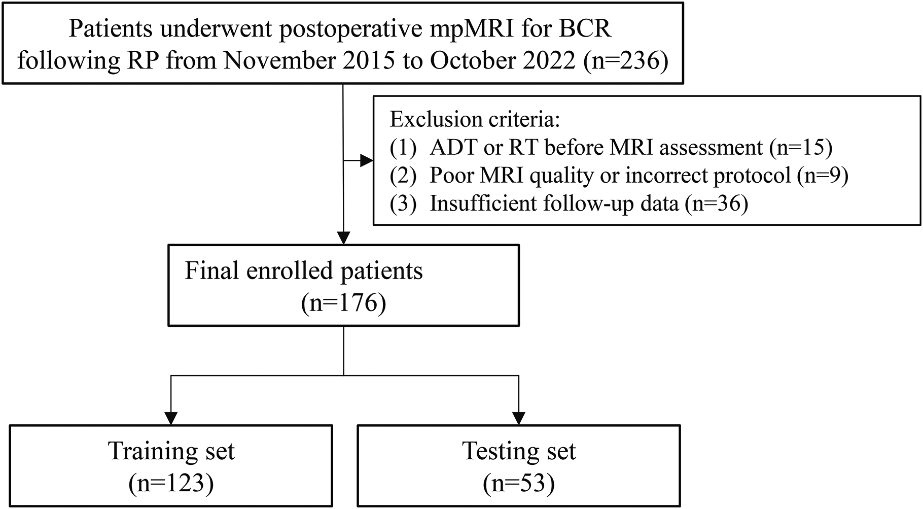
Patients with hypoattenuating liver metastases in mCRC and mPA that were examined in a 16-slice CT-scanner (Siemens Somatom Emotion, Siemens Healthcare GmbH, Erlangen, Germany) in our institution between 2011 and 2020 were identified retrospectively by the search terms “rectal cancer” and “pancreatic cancer.“ Only scans that were reconstructed in B30s Kernel with 1.5 mm slice thickness in axial orientation and acquired in portal venous contrast enhancement phase (60 s delay, 90 ml intravenous Imeron® (Bracco Imaging, Milan, Italy), 2.5 ml/s flow) were included. Based on our inclusion criteria, 47 mCRC patients and 31 mPA patients were included. In the mCRC population, 36.2% of the patients were female and had a median age of 64. Compared to that in the mPA collective, 51.6% of the patients were female and had a median age of 65.39. The patient characteristics for both groups are summarized in Table 1. The study protocol is summarized as a CONSORT diagram in Fig. 1.

Table 1 Patient characteristics. Median and IQR Fig. 1

Consort flow diagram showing the search terms, cohort selection criteria and structure of following analysis

Liver and lesion segmentation

To minimize the effect of inter-rater variability and create comparable results, a manual approach was chosen [19, 20]. Liver and liver lesions were segmented fully automated using the Applied Computer Vision Lab (ACVL) nnUNet pretrained liver segmentation model [21]. The created segmentations were corrected, if necessary, by a medical student (H.T., two years of experience in radiological image segmentation). Afterward, they were reviewed by a clinical radiologist (M.F.F. with more than four years of experience in oncologic imaging). The metastases segmentation mask was split into single lesion masks using 3DSlicer (version 4.11.20210226) [22]. Lesions smaller than 0.5 cm were considered too small to characterize and excluded. The liver tumor burden, defined as the ratio of metastasis to total liver voxel volume, was estimated by the automated segmentation.

Split into train, (validation), and test dataset

To evaluate the model’s performance, for both approaches eight patients with four from each group (mPA and mCRC) were randomly selected without stratification as an independent test set. The metastases image slices and radiomics signatures of these patients were not used during the training process. For the DenseNet-121 the dataset of cropped metastases CTs was randomly split into train, validation, and test sets in a ratio of 68/5/8 patients. If a patient had multiple liver metastases, all were only included in one set.

Radiomics-based classifiers

Radiomics features were extracted from the original images without filtering for patients with mPA and mCRC for each liver lesion using pyradiomics (version 3.0.1) [23]. Corresponding settings can be found in the supplementary material S1. First-order, 2D, and 3D shape features, neighboring gray tone difference (NGTDM), gray level co-occurrence matrix (GLCM), gray level run length matrix (GLRLM), gray level size zone (GLSZM), and gray level dependence matrix (GLDM) features were extracted. Following, the features were selected by applying a Pearson Correlation Coefficient (PCC) threshold of 0.6 for redundancy reduction. To identify the important features for the differentiation of metastases by primary, permutation-based feature importance was calculated using a Random Forest (RF) classifier. To account for imbalances in the input dataset, the synthetic minority over-sampling technique (SMOTE) using the python package imblearn (version 0.9.0) was performed on the training set. Random undersampling was used to investigate possible distortion of the input data by SMOTE. Standardization was applied to both the train and test set before analysis.

Several classification algorithms were implemented for the radiomics dataset: XG Boost (XGB), Random Forest (RF), Support Vector Machine (SVM), K-SVM, K-nearest neighbor, Logistic Regression, Naive Bayes, and Decision Tree. Hyperparameter tuning was performed if applicable to achieve maximum performance. Results from the test dataset were generated to compare lesion-wise performance.

Image-based CNN classifiersPreprocessing

The clinically diagnosed primary tumor for each patient was assumed as the ground truth for the corresponding liver lesions. To achieve a high degree of confidence, patients with multiple primary tumors were not enrolled. Automatically created segmentation masks were used to blacken the area surrounding the metastases, to only focus on the lesions. Following, the lesions were windowed in an abdominal window (window width of 330/window level of 10), cropped, and exported as images with a size of 224 × 224. Input images were augmented by zooming, shearing, rotation, and width shift and contained the entire lesion along with its borders.

Model definition and training

The model was trained from scratch using a DenseNet-121 for analysis, and single metastasis slices were used as an input. DenseNet-121 is a dense convolutional neural network algorithm with a depth of 121 layers [24]. The network for supervised learning was implemented in Pytorch. The analysis workflow is summarized in Fig. 2. Example lesions for colorectal and pancreatic liver metastases are displayed in Fig. 3. A detailed description of the model and training settings can be found in supplementary material S2.

Fig. 2

Technical pipeline for radiomics- and Densenet-121-based image slice analysis displaying used models and structure

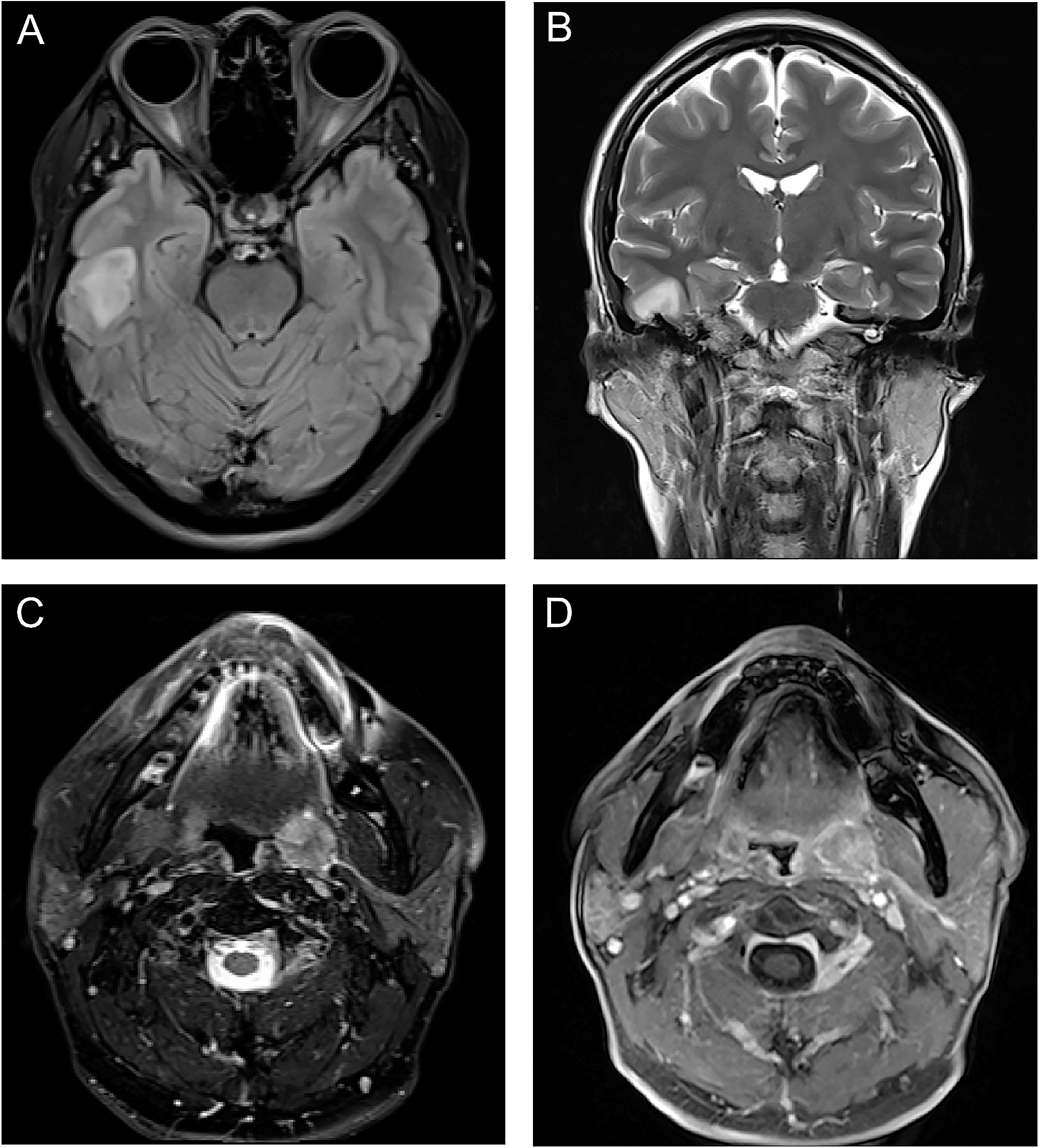
Fig. 3

Three example slices of visually indistinguishable liver metastases from each colorectal cancer and pancreatic cancer cohort

Lesion-wise comparison

To evaluate the performance on individual lesions, the slice-wise results were cumulated lesion-wise. The cumulated model outputs were classified as pancreatic or colorectal based on a cutoff value of 0.5.