Data source and study participants

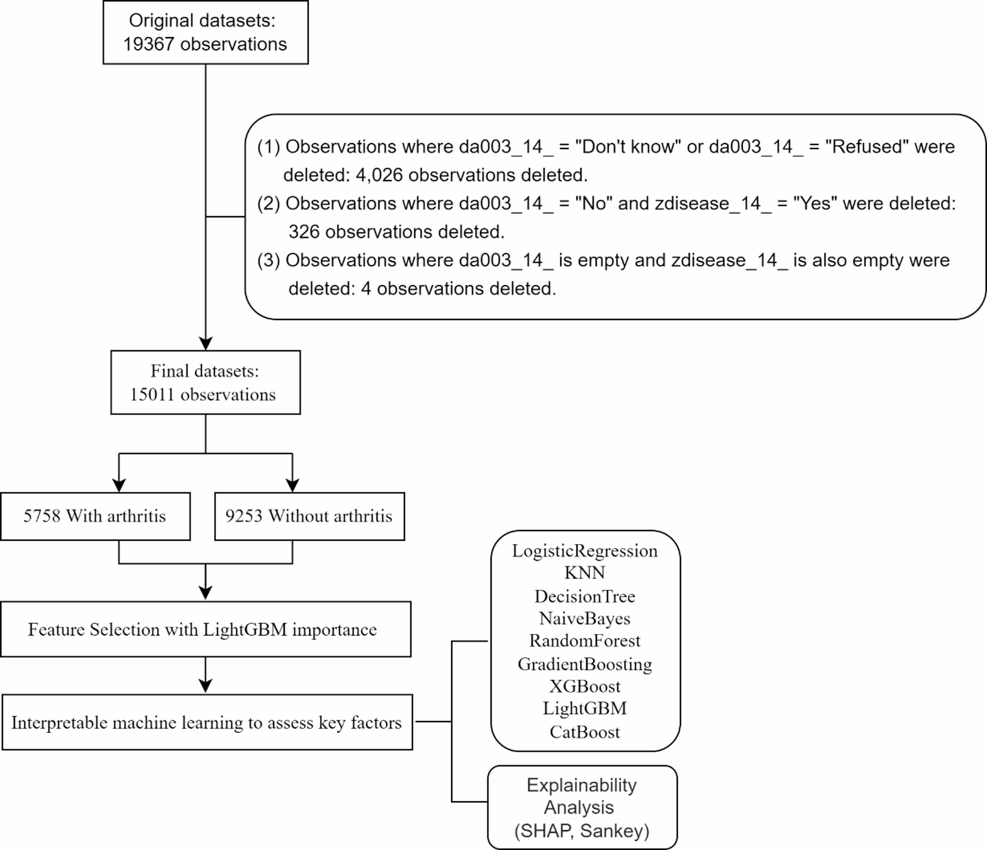
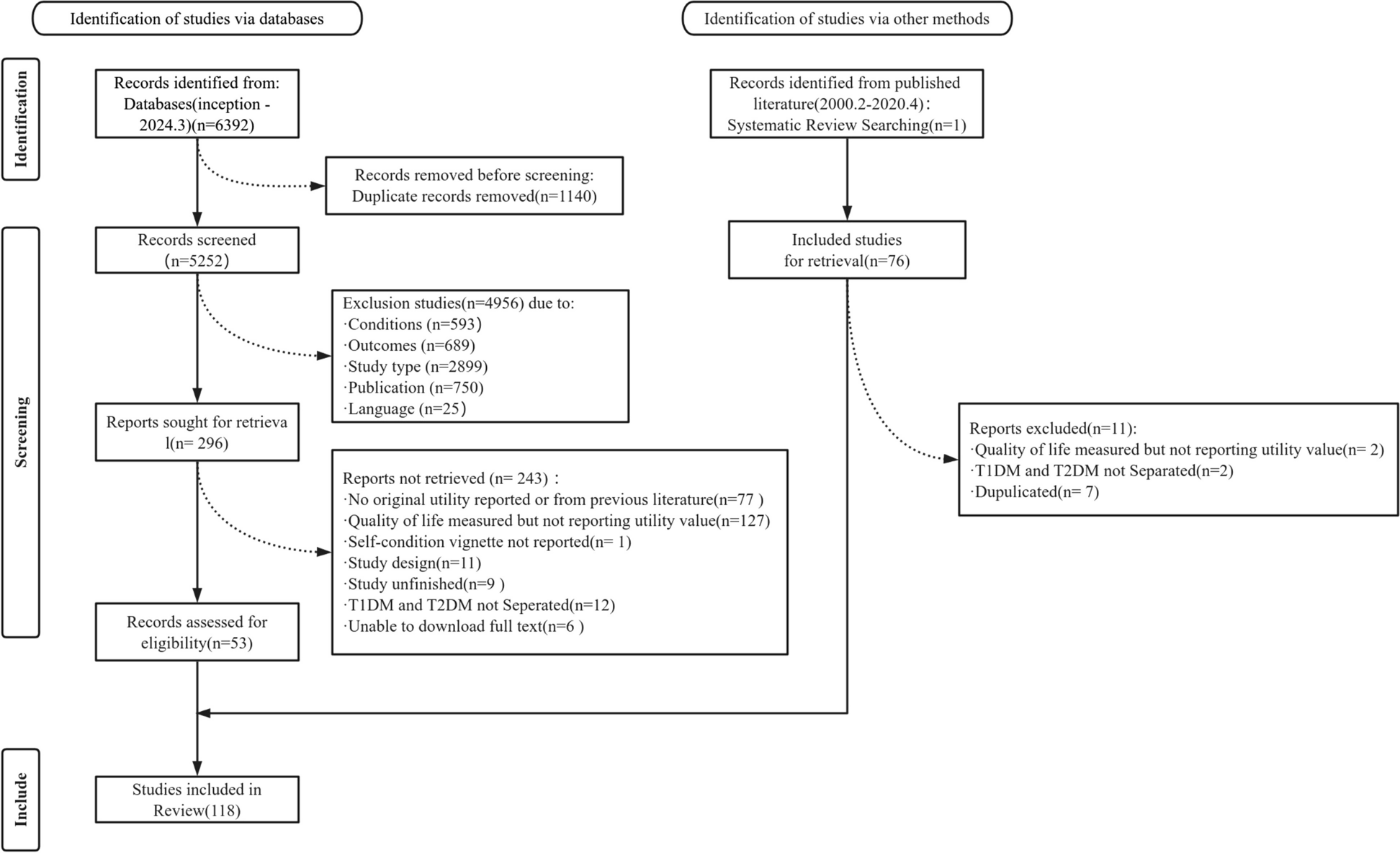
This study utilizes data from the 2020 CHARLS survey. CHARLS is a nationally representative longitudinal survey targeting individuals aged 45 years and older in China, with follow-up assessments conducted biennially since 2011 [21, 26]. The survey employs a multi-stage stratified probability proportional to size (PPS) sampling strategy to ensure sample representativeness [21]. Ethical approval for CHARLS was granted by the Biomedical Ethics Committee of Peking University (IRB00001052-11015.1.2), and informed consent was obtained from all participants [26, 27]. The initial dataset included 19,367 respondents. As illustrated in Fig. 1, after excluding records with inconsistent or missing responses to key diagnostic questions regarding arthritis, the final analytical sample comprised 15,011 individuals.

Fig. 1

The research design and data cleaning process

Variable selection and feature engineering

The outcome variable of this study was arthritis diagnosis (1 = yes, 0 = no), obtained from participants’ self-reported physician diagnoses recorded in the CHARLS survey. Based on standardized QoL scales (WHOQOL-BREF [12], SF-36 [13], and QLICD-RA [14]), we initially selected 55 potential predictive variables from the CHARLS 2020 dataset, covering various dimensions including demographic characteristics, health behaviors, self-rated health, functional limitations (ADL/IADL), pain, mental health, sleep quality, and social support (detailed in Appendix Table 1).

Further feature engineering yielded derived variables, such as aggregated scores (e.g., ADL/IADL difficulty counts, pain location count, cumulative positive/negative affect score), binary indicators (poor health status, need for assistance, inability to work due to health problems, pain interference), categorical variables derived from discretized continuous variables (age groups, sleep duration categories). To handle missing data, we also generated missing-value indicators. Specifically, for each original variable containing missing values, a corresponding binary indicator variable (1 for missing, 0 for present) was created. This approach allows the models to learn from any potential patterns inherent in the missingness itself. This entire process expanded the candidate feature set to 126 features.

Data preprocessing and feature selection

The dataset was randomly partitioned into training (70%, N = 10,507) and test sets (30%, N = 4,504) using stratified sampling. The overall data processing and feature selection workflow followed a five-stage pipeline to derive the final set of predictors:

1.

Initial Variable Selection: 55 potential predictors were initially selected based on established QoL domains (as described in Sect. 2.2).

2.

Feature Engineering: The set was expanded to 126 candidate features through the creation of aggregate scores and indicator variables.

3.

Data Preprocessing: This stage included imputation for missing values and standardization for numerical variables.

4.

Feature Space Expansion: One-hot encoding of categorical variables expanded the feature space to 133 dimensions ready for selection.

5.

Feature Selection: A data-driven selection using LightGBM importance rankings yielded the final 68 features for modeling.

A detailed account of this pipeline is as follows. We first applied a comprehensive preprocessing pipeline to the 126 candidate features. No variables were excluded based on a missing data threshold, as this could inadvertently eliminate important predictive information. Missing values were handled using a two-part strategy: the missing indicator variables created in the previous step were retained, and the original variables were imputed. Specifically, missing numerical values were imputed using the median (robust to outliers), while missing categorical values were imputed using the mode (most frequent value).

Subsequently, all categorical variables underwent one-hot encoding, which expanded the feature space from 126 to 133 final dimensions. All numerical variables were then standardized using StandardScaler [28]. Feature selection was then conducted using feature importance rankings from a LightGBM model. Figure 2 illustrates the top 30 most important features identified by the LightGBM model used for selection. Based on the median of feature importance scores across all 133 preprocessed features, a total of 68 features were ultimately retained for subsequent model training.

Fig. 2

LightGBM-Based Feature Importances (Top 30) Guiding Feature Selection

Model construction, validation, and interpretation

Nine ML models were evaluated: LogisticRegression, KNN, DecisionTree, NaiveBayes, RandomForest [29], GradientBoosting [25], XGBoost [30], LightGBM [22], and CatBoost [31]. This model portfolio spans the full spectrum from simple linear models to complex ensemble methods, enabling comprehensive evaluation of arthritis status prediction based on QoL-related features in the CHARLS dataset. To address class imbalance (arthritis prevalence of approximately 38%), Synthetic Minority Over-sampling Technique (SMOTE) was applied exclusively to the training data. Hyperparameter tuning was performed using Bayesian optimization (Optuna), targeting recall optimization through five-fold cross-validation. Detailed hyperparameter search spaces are provided in the Appendix Table 2.

Model performance was evaluated on the independent test set using multiple metrics, including AUC, AP, Recall, Specificity, Precision, and F1-score. ROC curves were generated to assess model effectiveness. For interpretability, SHAP was utilized to illustrate individual and collective feature contributions. Additionally, Sankey diagrams provided an intuitive visualization of the cumulative contributions of features to arthritis predictions.

All analyses were conducted in Python 3, utilizing the libraries pandas, NumPy, scikit-learn, imblearn, Optuna, XGBoost, LightGBM, CatBoost, dcurves, Matplotlib, and Seaborn. Statistical comparisons for baseline characteristics in Table 1 utilized Chi-squared tests. Statistical significance was set at p < 0.05.