Forty older healthy adults and thirty healthy young adults were recruited from the Free University of Tbilisi, Georgia. Detailed demographical information is presented in Table 1.

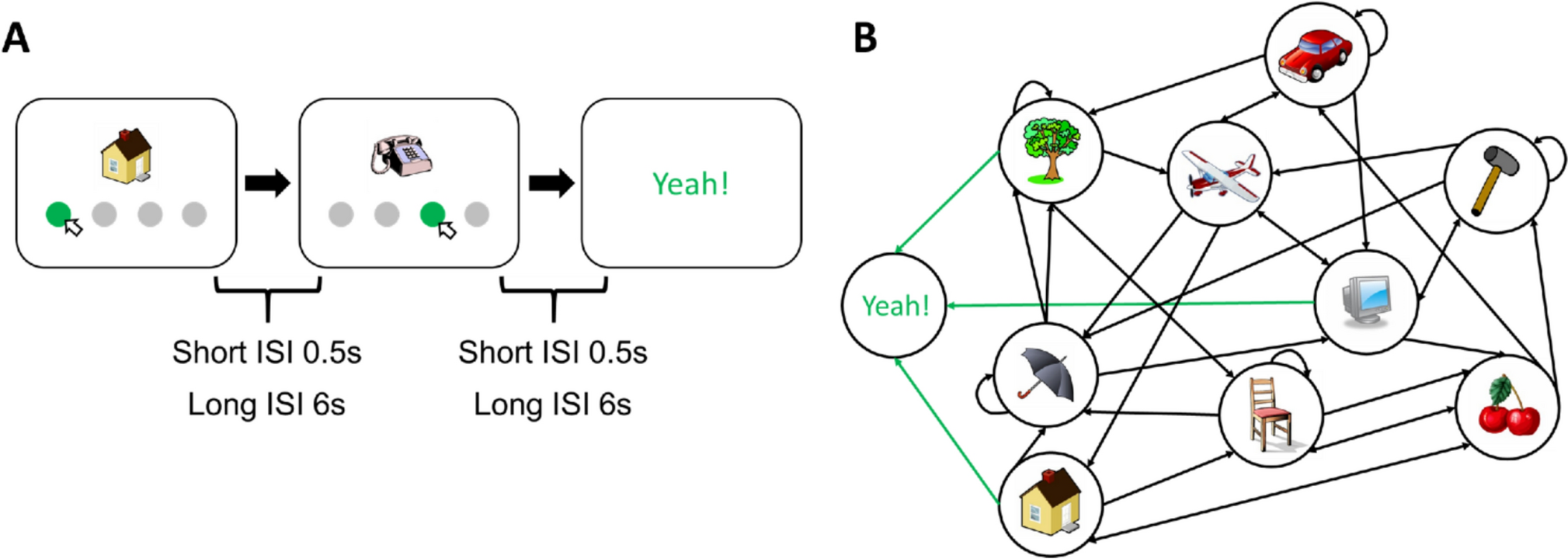
Participants performed a reinforcement learning task (Fig. 1). An image appeared in the center of the screen together with four gray disks below. Participants were instructed to choose and click on one of the disks. Clicking on a disk led to the presentation of the “next” image, with each of the four disks linked to a different subsequent image. The experiment resembles the above navigation task for finding food, where each decision (e.g., clicking on the right disk) leads to new images until a goal image is reached. In this respect, images correspond to states in RL terminology, and clicking on a disk corresponds to actions. The entire set of images/states constitutes an environment determined by a transition matrix that connects images/states via actions/clicks (Fig. 1B). During navigation through this environment, an “old” image could reoccur multiple times, resulting in participants navigating in a loop. When revisiting an old image, the grey disks led to the same next images as before. For example, whenever the tree image appeared, clicking on the left disk led always to the presentation of the image of a chair. Hence, it is crucial to learn the disk-next-image associations. There was no time limit for choosing a disk. The objective was to find a goal image, labeled with the word “Yeah!”. Before the start of the experiment, all nine possible images were presented on the screen, except for the goal image, which was not presented, but participants were informed about it. Participants initiated the experiment by clicking on a gray disk at the bottom of the screen. An episode consisted of the navigation process until the goal state was found. Participants started the next episode at a randomized location that was at least 2 steps away from the goal state. Furthermore, all these initial states were identical for all the participants.

We used two inter-stimulus intervals (ISI) of 0.5 s (short ISI condition) and 6 s (long ISI condition) between the participant’s responses and the next state, respectively. The objective of the task was to reach the goal state as frequently as possible within 8 min for the short ISI condition, and 30 min for the long ISI condition. The order of the two ISI conditions was counterbalanced among the participants, i.e., half began with the short ISI condition and the other half started with the long ISI condition. There is one transition matrix for each ISI condition, which was identical for all participants.

Twenty older healthy adults and twenty young healthy adults were recruited from the Free University of Tbilisi, Georgia. Individual who had previously taken part in the first experiment were no eligible. Detailed demographical information is presented in Table 1.

Experiment 2 follows a similar procedure as experiment 1, with the difference that, instead of a fixed duration of 8 min, the number of trials was fixed at 150 for each of the ISI condition. Accordingly, the objective of the task was to reach the goal state as many times as possible within the given number of trials. Furthermore, the order of the two ISI conditions was fixed, with the long ISI condition always coming after the short ISI condition.

Immediately after the RL task, a memory task was given to the participants. In total, there were eighteen images. Twelve of these images were the same as in the RL task, the other six images were novel. For each of the images, participants were asked (1) to indicate whether the given image appeared in the RL task, and (2) to rate their confidence in question one, on a 4-Likert scale.

In experiment 1, participants were instructed to reach the goal state as often as possible within 8 min. Due to the nature of the task, different observers visited a different number of images ranging from 30 to 200 due to differences in decision-making and reaction times. To ensure the comparability of the data among the participants, only the first 58 trials (the fifth percentile of the average number of trials among all participants) were used. Any trials exceeding this threshold were discarded. Four participants from the older population were removed from the study, as their total number of trials was lower than 59 trials. It is important to note that this pre-processing procedure only applied to experiment 1 as in experiment 2 the number of trials was fixed for all participants.

We determined the number of episodes completed and the proportion of optimal actions taken. The number of episodes completed refers to the number of times the participants reached the goal state. The proportion of optimal actions is the number of times a participant chose the that optimally reduced the distance to the goal state from the current state divided by the total number of actions performed in the task. To establish a performance baseline, we simulated an agent performing the task 1000 times, making completely random decisions. At each state, the agent chose an action with uniform probability. The baseline was determined by the average number of episodes completed and the proportion of optimal actions.

Furthermore, we assessed their improvement in performance by calculating the difference in the last and first 29 actions for the number of episodes completed and the proportion of optimal actions. A larger difference indicates better improvement, thereby implying enhanced learning. These four measures are our primary measures. Please note, these measures are not independent of each other. To gain further insights we used a number of secondary measures that are also not independent from the primary measures and can be seen as sub-measures.

First, the nine states of the environment were further categorized into adjacent and distant states. Adjacent states are states that were only one step away from the goal state. The six distant states were at least two steps away from the goal state. We analyzed performance separately for the two measures.

Second, to gain more insight into how performance progressed over time, we calculated the cumulative probability of optimal action across all trials. For each participant, we fitted a log function to estimate the intercept and the slope of the performance curve:

$$y=a+b*log \left(x\right)$$

\(x\) represents trial numbers, \(a\) and \(b\) are the intercept and the slope, respectively, \(y\) is the cumulative proportion of optimal actions in each trial.

Third, we tested perseveration behavior. It is essential to efficiently select the optimal actions for a given state in order to achieve superior performance. Choosing repeatedly a non-optimal action in a given is suboptimal and may be related to perseverative behavior or memory deficits. We determined perseverations in two ways. First, we determined the average length of repeating action sequences. We averaged the length of these repetitions of actions across all episodes for each participant. For instance, an episode with the actions “1,2,3,1,2,3,4,2,1” has an average perseveration of two because the action sequence “1,2,3” appeared twice. Second, we calculated the proportion of repeated state-action pairs. In an episode, we extracted all the states and the corresponding actions to determine the probability that the same state-action pair has been visited within the same episode. In order to be considered optimal, a state should not be visited multiple times within an episode.

Fourth we determined the action entropy, measuring the randomness of the actions chosen. The theoretical max entropy is

The probability distribution of completing each of the four actions was then determined for each state. The entropy of each state is

Here, i represents states, ranging from one to nine, while j represents actions, ranging from one to four. Averaging the action entropy across all states was computed for each participant. High action entropies indicate poor action choices (Sojitra et al. 2018).

Furthermore, we calculated the occupancy map for each state-action pair. Each cell in the matrices represents the number of times a participant engaged with a given state-action pair. Thus, a higher number in a cell indicates more frequent engagement with that specific state-action pair by the participant. Consequently, each participant will have two maps: one for the short ISI condition and one for the long ISI condition. To assess the similarity between these two maps for each participant, we used the cosine distance, calculated as follows:

$$}\;} = - \frac^ A_ B_ }}^ A_^ } *\sqrt ^ B_^ } }}$$

where \(A_\) and \(B_\) are the elements of vectors A and B, respectively, with each element corresponding to the occupancy counts for a specific state-action pair. Given that there are nine different states and four possible actions from each state, the total number of unique state-action pairs is 36.

A Q-learning model (Sutton and Barto 2018) was used to quantify learning:

$$\left(S,A\right)\leftarrow Q\left(S,A\right)+\alpha \left(\Delta \right)$$

S represents the state of the current trial, A is the action taken in the current trial, \(\Delta\) is the prediction error, Q is the Q-value for the given state and action, and \(\alpha\) is the free parameter of the learning rate. Whenever a participant performed a new action, the Q value was updated by the prediction error, which is defined as the difference between the current reward and the expected reward:

$$\Delta = r+\underset}Q\left(_,_\right)-Q\left(S,A\right)$$

r stands for the reward, \(_\) is the new state after performing action A in the given state S. The probability of choosing an action is then determined by a soft-max rule:

$$q\left(S,_\right)=\frac^_\right)}}}_^_\right)}}}$$

q is the probability of choosing action A given state S. \(\tau\) is the free parameter normally referred to as inverse temperature which corresponds to the exploration rate.

We conducted a two-by-two repeated measures ANOVA with age group (old and young) and ISI (short and long) as independent variables. We quantified the relationship between measurements using Pearson correlations, except for the relationship between measurements and Q-learning model parameters, which were calculated with Spearman’s correlation due to the non-normal distribution of the parameters.

The primary parameters, focusing on performance, learning, and Q-learning model in RL, are presented in the main text. The secondary parameters, are found in the supplementary figures. All details are summarized in Tables S1, S2, and S3.