1 Introduction

With the continuous development of electronic information technology, robots, as a key carrier in the realm of artificial intelligence, have been assuming a progressively substantial role in manufacturing (Arents and Greitans, 2022), healthcare (Khan et al., 2020), service industries (McCartney and McCartney, 2020), and beyond (Cheng et al., 2023; Tanyıldızı, 2023; Yang et al., 2023; Liufu et al., 2024), bringing numerous conveniences to human life and work. Many scholars are focusing their attention on robotics research field.

A robotic arm is a mechanical device composed of multiple linked joints, typically equipped with various end-effectors based on the requirements of the work environment. By calculating and adjusting the rotational changes of each joint, the end-effector can be controlled to perform various movements in a predetermined manner, such as position and orientation, thereby accomplishing tasks. For instance, the MATLAB program and particle swarm optimization were utilized for the trajectory planning of the robotic arm (Ekrem and Aksoy, 2023); Chico et al. (2021) employed a hand gesture recognition system and the inertial measurement unit to control the position and orientation of a virtual robotic arm. A target admittance model was designed in the joint space for hands-on procedures that can be applied in all commercially available general-purpose robotic arms with six or more DOF (Kastritsi and Doulgeri, 2021).

Due to the escalating complexity of task environments, single robotic arms frequently encounter challenges in effectively completing tasks, which highlights the advantages of dual robotic arms in collaborative and efficient task execution. For example, Jiang et al. (2022) presented an adaptive control method for a dual-arm robot to perform bimanual tasks under modeling uncertainties. Bombile and Billard (2022) designed a unified motion generation algorithm that enables a dual-arm robot to grab and release objects quickly. Wang et al. (2023) proposed a sliding mode controller with good robustness against the model uncertainties to capture and stabilize a spinning target in 3D space by a dual-arm space robot.

However, some of the methods mentioned above do not take into account the actual physical constraints of the robotic arms during initial modeling (e.g., Bombile and Billard, 2022; Jiang et al., 2022). This greatly limits the application scenarios of these algorithms and is inconsistent with the real working conditions of the robotic arms. Furthermore, the physical limitations of robotic arms typically pertain to constraints on joint angle and velocity. These constraints do not reside at the same constraint level, thus there are substantial computational challenges when attempting to address them collectively. An optimal approach entails a series of conversion strategies to harmonize these distinct hierarchical constraints to a congruous level (Zhang and Zhang, 2013) (e.g., velocity level). By implementing this approach, the constraints can be effectively unified and dealt without compromising their intended meaning. Some scholars (e.g., Li, 2020) have crafted novel approaches to these conversion strategies stemming from this foundation. Nevertheless, in the process, they have introduced too many supplementary parameters, rendering the strategies less straightforward for apprehension. Additionally, certain studies focus on the control of dual robotic arms based on 2D space, considerably limiting the operating range of robotic arms (Stolfi et al., 2017; Yang S. et al., 2020; Yang et al., 2021).

In recent years, with the rapid advancement of neural network research, many scholars have been committed to applying its formidable nonlinear modeling capability and efficient parallel computing ability to the domain of robotic arm motion control (Wang et al., 2021; Jin et al., 2024). This endeavor has given rise to a special kind of neural network known as the RNN (Xiao et al., 2021; Yan et al., 2022; Fu et al., 2023). For example, Xiao et al. (2021) proposed a noise-enduring and finite-time convergent design formula is suggested to establish a novel RNN. Fu et al. (2023) presented a gradient-feedback RNN to solve the unconstrained time-variant convex optimization problem.

To facilitate the calculation on computers and other digital hardware devices, some scholars focus on discretizing conventional CRNN models through time discretization techniques, leading to the development of DRNN algorithms (Liao et al., 2016; Liu et al., 2023a,b; Shi et al., 2023). The technique of second-order Taylor expansion was used to deal with the discrete time-variant nonlinear system, and a DRNN algorithm was proposed subsequently (Shi et al., 2023). Liao et al. (2016) proposed two Taylor-type DRNN algorithms on account of the Taylor-type formula to perform online dynamic equality-constrained quadratic programming. Liu et al. (2023a) designed a Taylor-type DRNN algorithm based on Taylor-type discrete scheme with smaller TE. It is worth noting that higher accuracy requirements often make the discretization formulas more complicated, inevitably leading to a large amount of computation and increasing the cost of actual production applications. After overall consideration, this study proposes an adaptive DRNN algorithm based on a three-step general Taylor-type discretization formula with an adaptive sampling period introduced, which is of high enough precision for practical applications.

Typically, due to the use of fixed sampling periods and fixed convergence factors in the conventional DRNN algorithms mentioned above, it is difficult for them to achieve a balance in computational precision and convergence rate, resulting in limited algorithmic dynamic and convergence performance. Therefore, some researchers have tried to introduce various adaptive mechanisms into model/algorithm design (Song et al., 2008; Yang M. et al., 2020; Dai et al., 2022; Cai and Yi, 2023). For example, Yang M. et al. (2020) proposed two discretized RNN algorithms with an adaptive Jacobian matrix. Cai and Yi (2023) developed an adaptive gradient-descent-based RNN model to solve time-variant problems based on the Lyapunov theory. Dai et al. (2022) proposed a hybrid RNN model by introducing a fuzzy adaptive control strategy to generate a fuzzy adaptive factor that can change its size adaptively according to the RE. Song et al. (2008) proposed a robust adaptive gradient-descent training algorithm based on an RNN hybrid training concept in discrete-time domain.

In light of the aforementioned circumstances, this study formulates a DAPCMC scheme in 3D space based on the dual-arm robot system and the new JLCS. Subsequently, a novel ATT-DRNN algorithm with adaptive sampling period and adaptive convergence factor is devised to effectively face the challenge of achieving a dynamic balance between great computational precision and rapid convergence rate. When compared with the CTT-DRNN algorithm and the CET-DRNN algorithm, the proposed ATT-DRNN algorithm demonstrates outstanding computational precision and rapid convergence rate. To demonstrate the features and strengths of the proposed ATT-DRNN algorithm, Table 1 shows the comparisons among distinct methods for the motion control of robots.

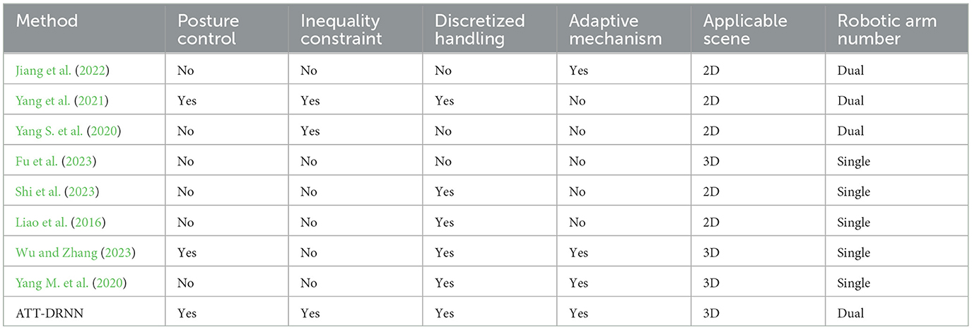
Table 1. Comparisons among distinct methods for motion control of robots.

The remainder of this study consists of four parts. Section 2 formulates the DAPCMC scheme and designs the ATT-DRNN algorithm. Section 3 presents the theoretical analyses of the proposed ATT-DRNN algorithm. Section 4 provides illustrative examples, and Section 5 concludes this study. Finally, the primary contributions/novelties of this paper can be summarized as follows.

1) Distinguishing from common dual-arm robot motion control schemes in 2D space, a novel construction methodology of the DAPCMC scheme in 3D space is provided, which can make a spatial dual-arm robot collaboratively execute repetitive tracking of a desired trajectory while adhering to a predetermined posture.

2) Distinguishing from existing strategies, an innovative JLCS is proposed, which has a ubiquitously differentiable and more succinct expression.

3) Distinguishing from conventional discretization methods, an innovative ATT-DRNN algorithm is engineered to address the DAPCMC scheme, which introduces a new adaptive convergence factor and sampling period to guarantee a notable convergence rate and exceptional convergence precision.

4) Distinguishing from the simple path-tracking task of single-arm robots, the posture collaboration motion control experiments of a UR5 dual-arm robot with the joint-angle and joint-velocity bound constraints considered substantiate the effectiveness of the proposed DAPCMC scheme and the outstanding convergence capability of the proposed ATT-DRNN algorithm.

2 Scheme formulation and algorithm design

This section describes how to construct a DAPCMC scheme that can be converted into a TVES problem and processed by the proposed ATT-DRNN algorithm.

2.1 Rudimentary knowledge

For the convenience of comprehension, let us construct a single robot arm motion control scheme with n DOF, which takes into account joint physical limits and can simultaneously ensure position control and orientation control during the MDRMC. Specifically, such a scheme can be described as below:

min.z˙(t) 12z˙T(t)U(t)z˙(t)+φT(t)z˙(t),    (1) s.t. J1(z(t))z˙(t)=Υ˙I(t)-α[ΥR(t)-ΥI(t)],    (2)  J2(z(t))z˙(t)=o˙I(t)-β[oR(t)-oI(t)],    (3)  z-≤z(t)≤z+,    (4)  z˙-≤z˙(t)≤z˙+,    (5)

where superscript T represents the transpose operator; z(t)=[z˙1(t),z˙2(t),...,z˙n(t)]T∈ℝn indicates the angle values of the robotic joints, and z˙(t)∈ℝn means the angular velocities of the robotic joints; matrix U(t)=In×n∈ℝn×n is an identity matrix; vector φ(t)=ξ[z(t)-z(0)]∈ℝn with design parameter ξ > 0 and z(0) means the initial joint-angle vector; J1(z(t))∈ℝ3×n and J2(z(t))∈ℝ3×n represent the position Jacobian matrix and the orientation Jacobian matrix, respectively; ΥI(t)∈ℝ3 and ΥR(t)∈ℝ3 represent the ideal path and the real position of the end-executor, separately; oI(t)∈ℝ3 and oR(t)∈ℝ3 represent the ideal orientation and the real orientation of the end-executor, respectively; α > 0 and β > 0 are both the error-feedback gains; z± and z˙± denote the upper and lower limits of z(t) and z˙(t), separately.

Remark 2.1: In accordance with previous experience (Zhang and Zhang, 2013), when t → ∞, the objective function (1) at the joint-velocity level is equivalent to ||z(t)-z(0)||22/2 at the joint-angle level, where the design parameter ξ > 0 ought to be adjusted as large as allowed by the manipulator conditions. Note that the robot arm's repetitive motion planning scheme under minimal displacement can be regarded as an optimization objective that can be resolved at the joint-velocity level.

Remark 2.2: Referring to the contributions of previous scholars (Yang et al., 2021), the equality constraint (2) at the joint-velocity level is equivalent to f(z(t))=ΥI(t) at the joint-angle level, when t → ∞ and the error-feedback gain α > 0 is at an appropriate value, where f(·):ℝn → ℝ3 represents the forward kinematics mapping function of a robotic arm.

Remark 2.3: Similarly, the equality constraint (3) at the joint-velocity level is equivalent to g(z(t))=oI(t) at the joint-angle level, when t → ∞ and the error-feedback gain β > 0 is at an appropriate value, where nonlinear function g(z(t))=oR(t)=[oRx(t),oRy(t),oRz(t)]T∈ℝ3 and the 2-norm of the real orientation vector oR(t) satisfies ||oR(t)||2 = 1.

Note that the inequality constraint (4) is at the joint-angle level of the system. In order to integrate inequality constraints (4) and (5) of distinct constraint levels into a unified formulation at the joint-velocity level as below:

℧-(t)≤z˙(t)≤℧+(t),    (6)

previous studies (Zhang and Zhang, 2013; Zhang et al., 2018; Li, 2020; Li et al., 2023; Qiu et al., 2023) supply a large number of JLCSs.

Nevertheless, the JLCS in Zhang and Zhang (2013) is unable to guarantee ℧−(t) or ℧+(t) to be differentiable anywhere. Meanwhile, as regard to the JLCS in Li (2020), ℧−(t) and ℧+(t) are designed as piecewise functions, respectively, and complex compound functions are embedded in them. In addition, the JLCS in Li et al. (2023); Qiu et al. (2023) adopt numerous design parameters and construct pretty complex expressions.

Therefore, as one of the contributions of this study, we provide a new JLCS. The ith (i = 1, 2, ..., n) elements of ℧−(t) and ℧+(t) in (6) are designed as follows:

where the corresponding parameters are all the same as in the previous section.

Besides, by taking into account the adaptive sampling period σk (37), the adaptive three-step general Taylor-type discretization formula can be expressed as follows:

ẋk=(-2a+1)xk+1+6axk-(6a+1)xk-1+2axk-22σk                                                             +O(σk2),     k=2,3,4,...,    (42)

Then, we can acquire the ATT-DRNN algorithm by using the adaptive three-step general Taylor-type discretization formula (42) to discretize the ACRNN model (41), which can be written as follows:

χk+1≐6a2a-1χk-6a+12a-1χk-1+2a2a-1χk-2-22a-1Mk[σk(-Vkχk-ϱk)-h(Hkχk+gk)],    (43)

where the solution step size h = σkζk is generally set at the range of (0, 1). Moreover, three initial state vectors χk with k = 0, 1, 2 are necessary to start up the proposed ATT-DRNN algorithm (43). The first one χ0 consists of ℧0, λ0, and μ0, where ℧0 is determined by the initial joint-velocity vectors of the LA and RA, while λ0 and μ0 are relatively arbitrarily set. The remaining initial state vectors can be generated by utilizing an adaptive Euler-type DRNN algorithm, which can be obtained by applying adaptive Euler forward formula to discretize the ACRNN model (41), i.e., χk+1≐χk+σkχ˙k with χ˙k=Mk[-Vkχk-ϱk-ζk(Hkχk+gk)].

Remark 2.5: By observing (37), it is evident that the adaptive sampling period σk continuously adjusts according to the changes in the RE ||ek||2, with an increase in the RE ||ek||2 and a decrease in the sampling period σk, and vice versa.

Remark 2.6: By observing (38), it is evident that the adaptive convergence factor ζk continuously adjusts according to the changes in the RE ||ek||2, when the RE ||ek||2 increases, the adaptive convergence factor ζk grows, leading to a higher convergence rate, and vice versa.

Remark 2.7: The solution step size h procured through multiplying σk and ζk is always a positive constant. By observing Equations (37) and (38) simultaneously, it can be easily found that σk and ζk exhibit the reciprocal states to each other. That is to say, when the RE ||ek||2 is large, the algorithm will adjust and yield a smaller sampling period σk and a larger convergence factor ζk to guarantee a rapid convergence of the algorithm in an extremely short sampling time; on the contrary, when the RE ||ek||2 reduces, the algorithm will adaptively increase the sampling period σk and simultaneously decrease the convergence factor ζk. By decreasing the sampling period and increasing the convergence rate, the algorithm can promptly complete the calculation and improve its computational efficiency. Therefore, the ATT-DRNN algorithm (43) can consider both computational accuracy and convergence efficiency during the calculation process.

3 Theoretical analyses and results

This section theoretically analyzes the convergence property of the ACRNN model (41) and the computational precision of the ATT-DRNN algorithm (43) for solving the TVQP problem (27)–(29).

Theorem 1: With the parameters h, p, q, δ > 0 of the continuous adaptive convergence factor ζ(t), the RE ||e(t)||2 generated by the ACRNN model (41) exponentially converges to zero in a large-scale manner with the exponential convergence rate at least being hpδ/q.

Proof: To begin with, by exploiting the EE (31), a Lyapunov function can be chosen as follows:

?(t)=||e(t)||222.    (44)

Then, the time derivative of the function ?(t) is obtained by referring to (40):

?˙(t)=eT(t)e˙(t)=-ζ(t)||e(t)||22.    (45)

Observing (44) and (45), one can draw the following conclusions.

(1) If and only if e(t) = 0, ?(t) = 0; otherwise, ?(t) > 0.

(2) If and only if e(t) = 0, ?˙(t)=0; otherwise, ?˙(t)<0.

In other words, the function ?(t) is positive definite and its derivative ?˙(t) is negative definite, which satisfies the Lyapunov stability theory conditions (Isidori, 1989). Thus, it can be concluded that the RE ||e(t)||2 converges to zero in a large-scale manner.

Second, by reconstructing and expanding (45), we acquire

?˙(t)=-2h(p+||e(t)||2)δq||e(t)||222=-2h(p+||e(t)||2)δq?(t).    (46)

Furthermore, based on (46), the following inequality can be further formulated as follows:

?˙(t)=-2h(p+||e(t)||2