Subjects and study site

Subjects were a total of N = 407 male rhesus macaques (Macaca mulatta) aged 1.17–20.7 years (mean ± SD = 3.30 ± 1.67). Subjects had been born and reared at the California National Primate Research Center (CNPRC) in Davis, CA. Subjects lived outdoors in any one of the 24 half-acre (0.2 ha) field corrals. Each corral measured 30.5 m wide × 61 m deep × 9 m high and contained up to 221 animals of all ages and both sexes. Subjects were tattooed as infants and dye-marked periodically to facilitate easy identification for husbandry- and research-related procedures. Monkeys had ad libitum access to Lixit-dispensed water. Primate laboratory chow was provided twice daily, and fruit and vegetable supplements were provided weekly. Various toys, swinging perches, and other forms of enrichment were provided in each corral, along with outdoor and social housing, thereby providing a stimulating environment.

The present investigation collated behavioral data obtained previously from five study cohorts (referred to below as Cohorts 1, 2, 3, 4, and 5). Subjects in these study cohorts had been selected independent of genetic relatedness, on the basis of the following criteria: male, socially housed in outdoor field corrals, medically healthy, not simultaneously enrolled in another CNPRC project, and previously enrolled in CNPRC’s BioBehavioral Assessment Program [33] as infants.

Reproductive management and parentage confirmation

The CNPRC houses approximately 4000 rhesus monkeys. A center-wide reproductive management plan has been in place for more than three decades to ensure an outbred colony. The formation of new corrals occurs regularly, and animals from multiple corrals are often combined to further prevent inbreeding. These decisions are guided by a geneticist. It was thus critical to determine the genetic parentage of subjects, which was accomplished using an established panel of microsatellite markers designed to identify maternity and paternity [34, 35].

Rank ascertainment

An individual’s rank may impact social behavior in nonhuman primates [36]. We therefore included subjects’ rank in the present study, and used the rank information that most closely corresponded to each subject’s behavioral data collection period (see below). CNPRC behavioral management personnel assess monkey ranks in each corral by recording aggressive and submissive interactions following food provisioning. Rank is ascertained on an approximately monthly basis beginning when animals are 2–3 years of age. Because each corral contains a different number of animals, rank is calculated as the proportion of relevant animals in the group that the focal individual outranks, such that the highest-ranked individual has a value of 1 and the lowest-ranked individual has a value of 0 [37]. Rank of course can impact young animals under CNPRC’s age threshold for ascertainment. Rhesus macaques maintain a despotic linear hierarchy [38], and early in life infants assume the rank of their mothers. Thus, for all subjects too young to receive a rank by behavioral management, we assigned the mother’s rank to these subjects. In Cohort 1, all subjects were old enough to have been assigned their own rank in the male hierarchy, whereas in Cohorts 2–5, a subset of subjects were young enough to still retain their mother’s rank. This necessitated that we calculate the proportion of individuals outranked slightly differently between study cohorts to ensure the most accurate ascertainment of a subject’s rank within them. Rank was accordingly Z-scored within each study cohort for use in the present study.

Behavioral observations and non-social equivalence score calculation

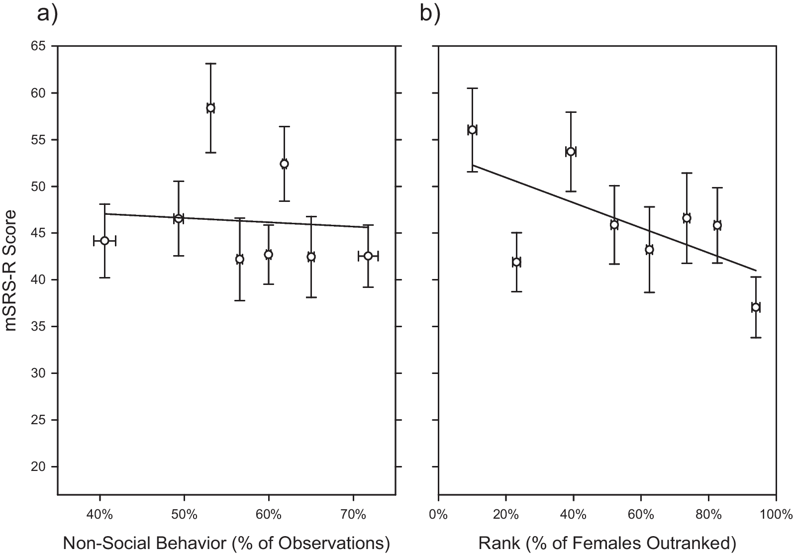
Unobtrusive behavioral observations had been previously conducted on N = 376 subjects from four of the five study cohorts (i.e., Cohorts 1, 2, 3, and 4) while they were in their home field corrals as previously described [19, 20, 23]. For Cohorts 1, 3, and 4, observers conducted 10-min focal samples on subjects during two observation periods per day, 4 days per week, for 2 weeks. The behavior of individual monkeys was recorded at 30-s (Cohort 1) or 15-s (Cohorts 3 and 4) intervals using instantaneous sampling. For Cohort 2, we adopted a scan sampling approach, enabling us to score multiple animals in the same group at the same time. Each observer conducted scan samples for a given corral during two observation periods per day. In each observation period, scan sampling was conducted at 20-min intervals, at a rate of 18 scans per day, for a total of five days. During each scan, the subjects in each corral were identified, and observers then recorded the behavior. The same five social behaviors were recorded for all study cohorts (i.e., the ethogram was the same regardless of sampling technique): non-social (subject is not within an arm’s reach of any other animal and is not engaged in play), proximity (subject is within arm’s reach of another animal), contact (subject is touching another animal in a nonaggressive manner), groom (subject is engaged in a dyadic interaction with one animal inspecting the fur of another animal using its hands and/or mouth), and play (subject is involved in chasing, wrestling, slapping, shoving, grabbing, or biting accompanied by a play face [wide eyes and open mouth without bared teeth] and/or a loose, exaggerated posture and gait; the behavior must have been deemed nonaggressive to be scored). Both sampling methods estimate the durations of behavior [39]. After completion of data collection, the total frequency of non-social behavior was then summarized across all of the behavior samples collected for each subject. As three of the study cohorts had been observed using instantaneous sampling methods with varying sampling intervals (i.e., Cohorts 1, 3, and 4), and one study cohort had been observed using scan sampling methods (i.e., Cohort 2), we created a “non-social equivalence score” by Z-scoring non-social behavior frequency within each study cohort to enable comparison of animals across different cohorts following [17].

mSRS-R ratings

mSRS-R scores had been previously obtained on N = 264 subjects from three of the five study cohorts (i.e., Cohorts 3, 4, and 5). Observers rated each subject on a 36-item original mSRS [25], which we had modified from a four-point to a seven-point Likert scale (1 = total absence of the trait, 7 = extreme manifestation of the trait) for each item. Prior to final summary, questions written in the infrequent direction were reverse scored such that higher scores always indicated greater impairment. Since only 17 of the original 36 mSRS items exhibited consistent inter-rater and test–retest reliability, we extracted and tabulated ratings for the 17 reliable items, which form the basis of the mSRS-R [19]. Ratings had been obtained using the same scale across study cohorts, so the mSRS-R ratings did not require normalization.

Data processing and statistical analyses

We first collated all available data for each subject. As noted above, measures that differed in the observation or calculation method between study cohorts (namely non-social behavior score and rank) were Z-scored within cohort prior to analysis, whereas measures that employed the same ascertainment method across study cohorts (namely mSRS-R score and variables such as age) were not Z-scored. A small number of subjects had been studied twice (i.e., they had been members of two different study cohorts). For these animals, we uniformly discarded their earliest data and retained their most recent data for analysis here.

We then used CNPRC’s multigenerational pedigree records to identify the father and mother for each subject. These data included a small number of full-sibling pairs. For our initial analyses, we uniformly discarded the youngest animal of the full-sibling pair to enable retention of one animal (the eldest) for the half-sibling analyses. Using the same pedigree data, we measured the inbreeding coefficient (F) for 40 random offspring as well as both of their parents. We also estimated the coefficient of relatedness (r) between each of these animals with every other animal included in this subset. While F is defined in terms of the probability of identity in state of different pairs of alleles, r measures the probability that alleles drawn at random from the same locus in each of two subjects will be identical by descent [40, 41]. Differences between sires and dams in these measures were tested by Mann–Whitney.

For the two behavior measures (i.e., the non-social equivalence score and mSRS-R score) we then generated two new datasets, and calculated the number of paternal half-siblings and the number of maternal half-siblings for each subject independently for each measure. Subjects with no paternal and no maternal half-siblings were then removed in each dataset. Thus, in each dataset each subject had at least one maternal or paternal half-sibling, and no full-siblings [42, 43].

Restricted Maximum Likelihood (REML) mixed models with unbounded variance estimates were used to estimate the variance components needed to calculate the genetic contribution of parents as the proportion of phenotypic variance (σ2P) between sons that could uniquely be attributed to their shared genetics (σ2g), expressed as σ2g/σ2P (or the proportion of phenotypic variance attributable to genetic variance), and narrow sense heritability (h2) following [15]. The individual genetic contribution of a parent is given as Best Linear Unbiased Predictors (BLUPs), generated in the same mixed models [15].

Different genetic scenarios have different dynamic ranges and expected values for σ2g/σ2P [15]. For instance, σ2g/σ2P in half-siblings given unimprinted autosomal effects has a maximal value of 25%, but imprinted genes (which are selectively silenced when inherited from the mother or father) increase σ2g/σ2P for one parent and decrease them for the other. Furthermore, variance estimates for mothers and fathers can be tested against each other. Thus, σ2g/σ2P captures more information than a traditional estimate of narrow-sense heritability (h2), despite the two measures being mathematically related [44, 45]. Absolute values of h2 are influenced by a wide range of effects, which combined with its strict definition in terms of purely additive haplotypic gametic contribution, limit interpretation. By focusing on additive genetic variance, and gametic potential, h2 essentially assumes that allele–allele interactions (e.g., dominance), gene–gene (e.g., epistatic) interactions, and gene–environment interactions (e.g., phenotypic plasticity) are not contributing to estimates of genetic variance. However, this is rarely the case, and so dominance and epistatic effects tend to inflate h2, whereas phenotypic plasticity can inflate or deflate it, depending on study design [42, 43]. Furthermore, h2 does not imply genetic determinism [42]: for example, h2 is often far higher than concordance rates [43], and often exceeds its theoretical limit of 1. Accordingly, we primarily present the results as σ2g/σ2P, which is broader but more meaningful in interpretation, has distinct meanings within its dynamic range, and cannot exceed its theoretical limits.

A critical advantage of this approach is that potential confounding environmental effects can be included in the model, and the variance components representing the half-sibling group (i.e., father or mother), are estimated after these confounds are taken into account (i.e., they are the estimate of the unique variance that cannot be explained by other terms in the model [30]). All mixed models included rank, age, and number of males in the social group to control for these potential influences on social behavior. Father and mother were included as random effects to calculate variance components. Furthermore, because each subject (son) belonged to a unique combination of paternal half-sibling group and maternal-half-sibling group, calculating father and mother variance components in the same model eliminated any possibility that shared environmental effects inflated our variance component estimates. Thus, if the son’s social behavior was driven by a shared environmental effect, mother would have no unique explanatory variance once father was taken into account, and vice-versa [46]. The power of this approach is that shared environmental confounds are controlled for universally and agnostically even if we do not know what they are [30, 46]. To test whether the variance components attributed to father and mother differed (and, hence, ultimately the σ2g/σ2P and h2 attributed to each), we used an F-test of the variance components with their respective degrees of freedom. The variance of σ2g/σ2P was calculated and used to calculate a Z-score and associated P value following [15]. Given the relationship between the σ2g/σ2P and h2, h2 shares the same Z-score and P value.

Best practice in linear (and mixed) model design is to stress-test the models to detect potential confounding effects (i.e., “orthogonality checks” or “sensitivity analysis” [46, 47]). In this case, we wanted to ensure the variance attributed to fathers and mothers in the analysis above held up when paternal and maternal half-sibling groups were analyzed separately. For these secondary analyses, the datasets for each social behavior measure were further subdivided and trimmed into datasets where every subject had at least one paternal half-sibling, or at least one maternal half-sibling, respectively. The same mixed models as described above were used, but now with only father or mother included. Processing of the variance components to σ2g/σ2P, h2, and their tests was performed as described above.

In the non-social equivalence score and mSRS-R datasets, 11 (4.0%) and 7 (3.6%) of the subjects, respectively, were not raised by their birth mother (e.g., because of kidnapping), yielding a total of N = 12 unique animals. To ensure that these subjects were not introducing an artefact, we repeated the analyses above excluding these individuals. Doing so did not change the results. We therefore present the analyses from the full data sets, especially as doing so is the conservative biological and statistical approach (i.e., retaining these subjects should, if anything, reduce the impact of environmental confounds on the final results).

Finally, given the apparent selective genetic contribution from fathers but not mothers, we generated a trimmed dataset for full-siblings. Full-siblings are rare given the rhesus monkey’s promiscuous breeding system. Nevertheless, we were able to analyze full-sibling data for one of our measures: the non-social equivalence score (N = 24). The same mixed models were used to generate variance components, σ2g/σ2P, and h2. We did not have enough full-sibling pairs to calculate meaningful tests for the σ2g/σ2P, but we could test the variance component estimates against those from the half-sibling data. These F-tests enabled us to test whether full-siblings differed in the magnitude of their variance components (and hence σ2g/σ2P) from paternal and maternal half-siblings.

σ2g/σ2P, h2, and variance components are population-level summaries, and are not readily visualized. Therefore, for visualization purposes we calculated the predicted genetic contribution of each father and mother (also referred to as the “breeding value”) as the BLUP, which is given as the deviation from the population average.

Mixed models were performed in JMP 15 Pro for Windows. Further calculations of σ2g/σ2P, significance tests of σ2g/σ2P, and calculation of h2, involved several further steps [15] and were performed in Excel.

Note that this statistical approach is essentially equivalent to an “Animal Model” [30] with a pedigree cut at the parental level. The main advantage of the “Animal Model” is its ability to extract additional information from complex pedigrees by comparing individuals with different relatedness in multiple layers of the pedigree. This advantage, however, is minimal here, as we are only comparing siblings, and almost all are half-siblings. Moreover, the cost of implementing the “Animal Model” here is substantial, as it necessitates a range of requirements and assumptions (e.g., a balanced mixture of half- and full-siblings) that cannot be met by this data set, and carries a risk of false negatives due to confounding variables [30]. We therefore chose to adopt the well-established and simpler statistical approach described above.