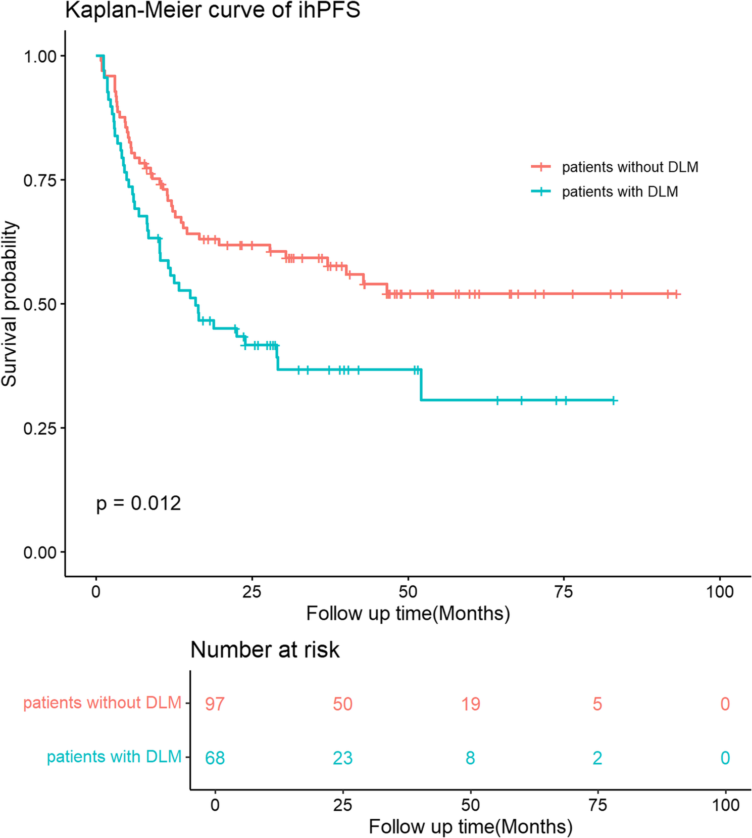
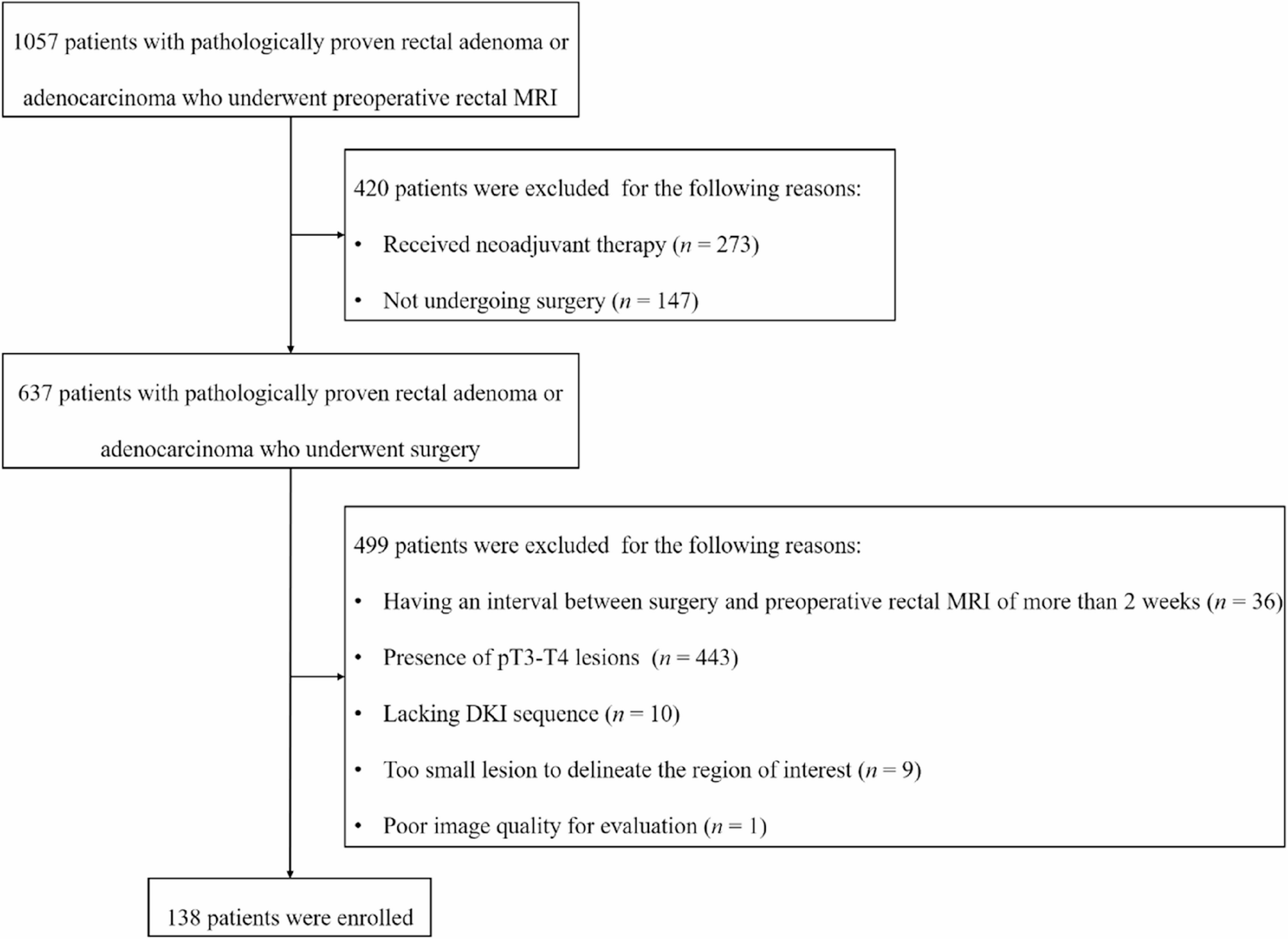
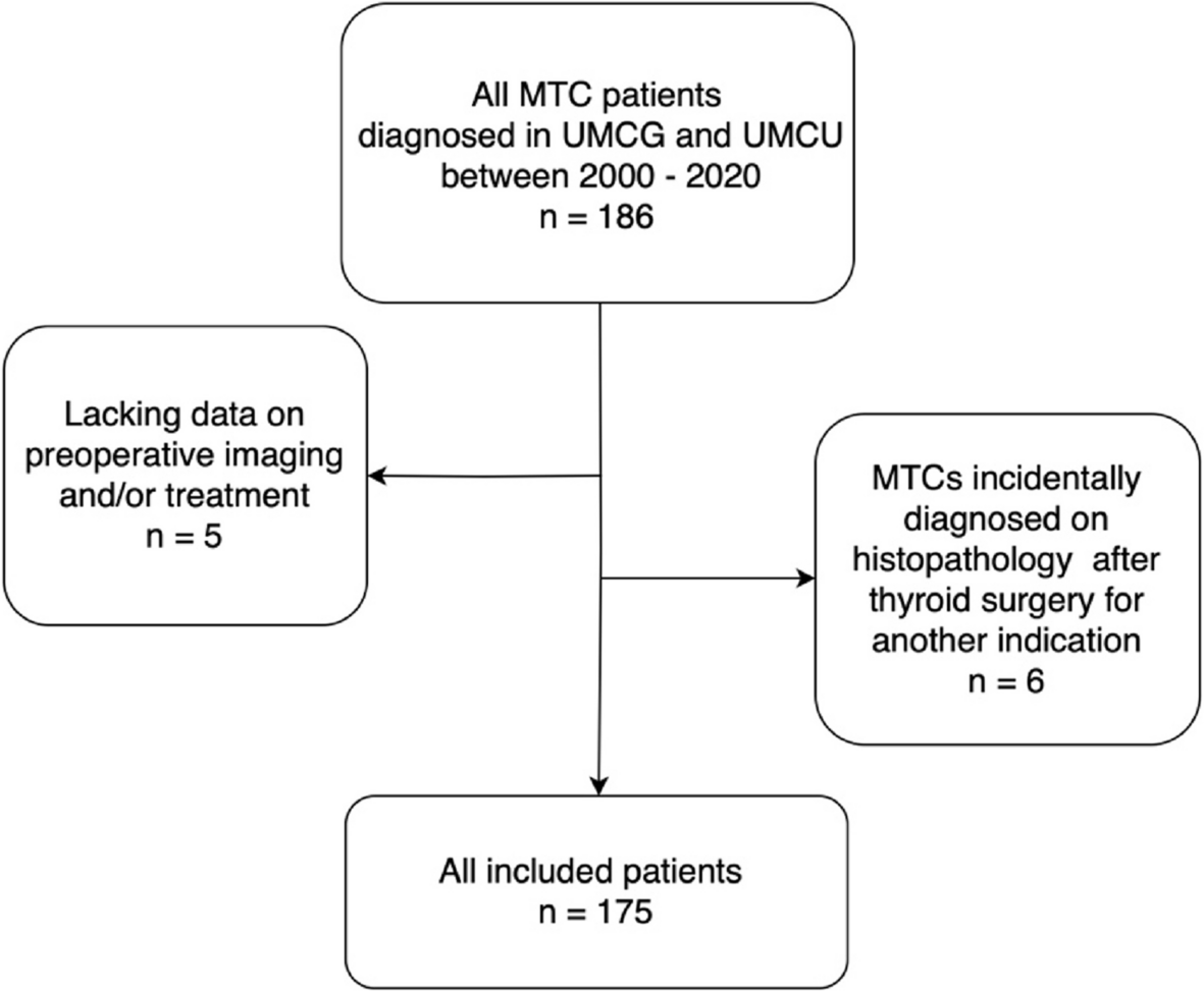
This retrospective study was approved by our Institutional Review Board (IRB No. [2025]455) with a waiver of informed consent. A total of 1057 consecutive patients with pathologically confirmed rectal adenoma or adenocarcinoma who underwent preoperative rectal MRI were collected from January 2018 to December 2023. Patients were excluded for the following reasons: (a) received neoadjuvant therapy (n = 273); (b) not undergoing surgery in our hospital (n = 147); (c) having an interval between surgery and preoperative rectal MRI of more than 2 weeks (n = 36); (d) having a postoperative pathological T stage > T2 (n = 443); (e) lacking DKI sequence (n = 10); (f) having a lesion that was too small to delineate the region of interest (n = 9); (g) poor image quality for evaluation, such as metal and motion artifacts (n = 1). Finally, 138 patients were enrolled (mean age, 60 years ± 12 [standard deviation]; 79 male) (Fig. 1).

Flow diagram of patients’ enrollment

To enhance the visibility of the tumor, an appropriate amount of gel (20–80 mL) was rectally administered based on the tumor location determined by colonoscopy or CT. To minimize artifacts related to intestinal peristalsis, 20 mg of raceanisodamine hydrochloride (MINSHENG PHARMACEUTICAL Co., Ltd.) was administered intramuscularly approximately 10 min before the MRI examination, unless contraindicated.

The images were acquired using a 3.0 T MRI scanner (Magnetom Verio; Siemens Healthineers) with a 6-channel phased-array surface coil in combination with the built-in spine coil. The rectal MRI protocols included (a) axial T2WI using a turbo spin-echo sequence; (b) sagittal, coronal, and orthogonal axial (perpendicular to the tumor base) HR-T2WI using a turbo spin-echo sequence; and (c) axial diffusion imaging using a single-shot echo-planar imaging sequence with b values of 0, 200, 600, 1000, 1500 and 2000 s/mm2 (Table 1).

Two radiologists (Y.C., Y.R.M; 9 and 6 years of experience in rectal MRI, respectively), who were unaware of the pathological results, independently reviewed HR-T2WI to determine the depth of tumor invasion. Tumors confined to hyperintense submucosa were defined as mrT1, while tumors infiltrating muscularis propria with loss of interface between submucosa and muscularis propria were classified as mrT2, and tumors extending beyond muscularis propria into perirectal fat with a nodular margin were categorized as mrT3 [20]. In this study, our aim was to evaluate the diagnostic value in determining pT0-T1 rectal tumors. Therefore, tumors diagnosed as ≥ mrT2 were grouped together. The discrepant findings between the two radiologists were resolved by a third gastrointestinal radiologist with over 20 years of experience (S.P.Y.).

All diffusion imaging data were imported into the post-processing software (MR Body Diffusion Toolbox v1.3.0; Siemens Healthineers).

Based on the DKI model, b values of 0, 200, 600, 1000, 1500 and 2000 s/mm2 were selected. The kurtosis map and diffusivity map were calculated using three-variable linear least squares fitting with the following computation formula:

$$\:ln(S_b)=ln(S_0)-b\cdot\:D+1/6\cdot\:b^2\cdot\:D^2\cdot\:K$$

where Sb represents the MR signal intensity at specific b values; S0 represents the MR signal intensity when the b value is 0; D is diffusivity and quantified in mm2/s; K is kurtosis, which is a dimensionless metric.

The b values of 0 and 1000 s/mm2 were selected based on the DWI model, and the ADC map was calculated using the two-variable linear least square method. The calculation formula is as follows:

$$\:ln(S_b)=ln(S_0)-b\;\cdot\:ADC$$

where Sb represents different b values of MR signal intensity; S0 indicates the MR signal intensity when b value is 0; ADC represents the apparent diffusion coefficient in mm2/s.

The two radiologists (Y.C., Y.R.M.) independently performed slice-by-slice manual delineation along the tumor margins to encompass the entire tumor volume that exhibited high signal intensity on high-b-value diffusion images, using axial T2WI as a reference. The regions of interest were then copied to kurtosis, diffusivity, and ADC maps (Figs. 2 and 3). The kurtosis, diffusivity, and ADC values for all regions of interest, as delineated by two radiologists, were averaged for each patient to facilitate statistical analysis.

A 66-year-old male with pT1 rectal cancer. a Axial T2WI shows the tumor located along the right posterior wall of the rectum (white arrow). b The high-b-value diffusion image shows high-signal-intensity tumor (white arrow). ADC map (c), color-coded kurtosis map (d), and color-coded diffusivity map (e) (green line) show values of 1.088 × 10−3 mm2/s, 0.802 and 1.623 × 10−3 mm2/s, respectively. T2WI, T2-weighted imaging; ADC, apparent diffusion coefficient

A 59-year-old female with pT2 rectal cancer. a The tumor is located in the right anterior wall of the rectum on axial T2WI (white arrow). b The high-b-value diffusion image shows high-signal-intensity tumor (white arrow). ADC map (c), color-coded kurtosis map (d), and color-coded diffusivity map (e) (green line) show values of 1.102 × 10−3 mm2/s, 0.972 and 1.306 × 10−3 mm2/s, respectively. T2WI, T2-weighted imaging; ADC, apparent diffusion coefficient

All patients underwent surgery. The pathological reports concerning tumor and lymph node staging, derived from resected specimens, were based on the criteria of the American Joint Committee on Cancer and served as the reference standard.

Statistical analyses were conducted using SPSS software (version 26.0; IBM) and MedCalc statistical software (version 15.8; MedCalc Software bvba; https://www.medcalc.org; 2015). The normality of the data was tested using Kolmogorov-Smirnov test. Continuous data were described as means ± standard deviations or medians and interquartile ranges, and compared using independent samples t-test or Mann-Whitney U test. Categorical variables were reported as numbers and percentages, and compared using χ2 test or Fisher’s exact test. HR-T2WI-based T stage diagnosis, along with DKI and DWI parameters that showed a P-value < 0.1 in univariable analysis, were entered into multivariable logistic regression analysis using the ‘Forward: Likelihood Ratio’ method. Those variables that yielded a P-values < 0.05 in the multivariable analysis were subsequently incorporated into the combined logistic regression model. The receiver operating characteristic (ROC) curves were used to analyze the diagnostic value of significant indicators. The area under the ROC curve (AUC) was calculated, with the cutoff value determined by the maximum Youden index. AUCs was compared using the DeLong test. The intraclass correlation coefficient (ICC) was calculated to analyze the interobserver agreement for DKI and DWI parameters (ICC < 0.50, poor agreement; 0.50–0.75, moderate agreement; 0.76–0.90, good agreement; 0.91–1.00.91.00, excellent agreement) [21]. Interobserver agreement on the HR-T2WI diagnosed T stage was assessed using Kappa statistics (0–0.20.20 poor, 0.21–0.40 fair, 0.41–0.60 moderate, 0.61–0.80 substantial, and 0.81–1.00.81.00 perfect agreement). A two-tailed P value < 0.05 indicated statistical significance.