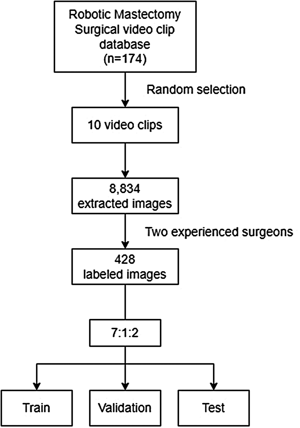
A total of 174 patients underwent RNSM using the da Vinci Si, Xi, or SP system between November 2016 and December 2020 at Severance Hospital. In the 174 patients, ninety-nine patients underwent RNSM using the da Vinci Xi system and 10 patients were randomly selected in the study. Clinicopathological data were collected from patients’ electronic medical records and video clips of the surgery. All patients were informed that a recorded surgical video could be used for academic research and educational purposes and signed a consent form. The video clips do not include any personal information of the patients. The ten videos had a spatial resolution of 1280 × 1024 pixels and a temporal resolution of 30.00 frames per second. Images were obtained by splitting each video into frames at 1-s intervals and converting them into the PNG format. Approximately 20,000 frames were initially extracted. To enhance quality, frames showing operating rooms or containing significant artifacts were manually identified and excluded, reducing the dataset to 8,834 frames. From the 8,834 extracted images, 428 images were selected after excluding images with high noise or without regions of interest (ROIs), and were divided into training, validation, and testing datasets at a ratio of 7:1:2. To ensure the dataset represented a diverse range of video content with minimal duplication, random sampling was employed. The surgical landmarks were marked by two experienced surgeons.

All RNSM procedures were performed by a single experienced breast surgeon with 23 and 10 years of experience in clinical practice and robotic breast surgery, respectively. Briefly, a skin incision was made anterior to the mid-axillary line below the axillary fossa. First, a sentinel lymph node biopsy was performed manually without robotic assistance using monopolar electrocautery or an advanced energy device, such as a bipolar energy vessel sealing device or ultrasonic shears. Second, the retromammary space was dissected, and tumescent solution was injected into the subcutaneous layer. After injecting the tumescent solution for hydrodissection, tunneling in the same layer was performed using Metzenbaum scissors and/or vascular tunnelers. Multiple tunnels were formed along the subcutaneous layer as landmarks for the dissection layer. A single port was inserted into the incision, and the robotic surgical system was docked. After docking, carbon dioxide gas was insufflated through a single port to expand and secure an operating space that included multiple tunnels, and video recording was initiated. The entire dissection of the skin flap was performed using the robotic surgical system. After the procedure, all breast tissues were retrieved from the incision site.

Two experienced surgeons marked the tunnels to create a surgical guide to accurately estimate the dissection planes of the skin flaps. One surgeon performed the RNSM procedure, and the other was a breast surgeon with 2 years of experience in clinical practice and robotic breast surgery. Two ground-truth references were created for each image, as each surgeon drew the tunnel manually using the ImageJ software. To achieve surgical guidance, an imaginary line was initially created by connecting the centers of the tunnels. The overall schematic is presented in Fig. 1.

Schematic flow of the current study

Upon reviewing the initial results, the researchers observed that the imaginary line was closer to the skin flap than to the actual dissection plane. To improve the guide, the imaginary line was revised by connecting the center of the tunnel bottom. The revised results were evaluated by two surgeons who labeled the prediction lines for skin flap dissection.

The proposed architectures comprised a modified EfficientDet (mEfficientDet) [12], YOLO v5 [13, 14], and RetinaNet [15]. The proposed architecture consisted of a convolutional neural net (CNN) with a mEfficientDetmodel. A schematic of EfficientDet-b0 is presented in Fig. 2(a). The structure of mEfficientDet uses EfficientNet [12] as the backbone (Fig. 2(a)), and the final structure, which uses a feature network, consists of four layers of BiFPN [16] stacked on top, which is a segmented prediction layer that predicts the target region pixel by pixel. EfficientNet, which is used as the backbone network, consists of several converged layers, MBConv blocks, and converged 1 × 1, pooled, and fully connected (FC) layers. In Conv 3 × 3, one convolutional layer was stacked with a 3 × 3 kernel and 32 channels, followed by one MBConv1 block with a 3 × 3 kernel and 16 channels, two MBConv6 blocks with a 3 × 3 kernel and 24 channels, two MBConv6 blocks with a 3 × 3 kernel and 40 channels, and three MBConv6 blocks with a 3 × 3 kernel and 80 channels. MBConv6 performs depth-wise batch normalization and sweep processes in MBconv. Finally, the FC layer is stacked, encompassing convolutional, pooling, and dense layers, using a 3 × 3 kernel. MBConv uses depth-specific convolutional layers. Unlike regular convolution, which affects all channels, depth-wise convolution partitions the feature map by channel and applies the convolution to only a single channel, which can exponentially reduce the computation. Subsequently, normalization was performed using batch normalization to adjust the mean and standard deviation of all inputs in the batch. A sigmoid-weighted linear unit (switch) was used for activation. A BiFPN is a type of fully convolutional network, where 1 × 1 convolutions act as FC layers. In particular, a BiFPN can be considered as a learning sequence and path through convolution. A segmentation logit is a network that handles the final goal region. The last layer in the BiFPN classifies the target region and processes the final prediction using a layer that handles the boundaries of the region. To supplement the current accuracy, we applied YOLO v5 (Fig. 2(b)) [17, 18], an object-detection algorithm that can detect objects faster with fewer parameters and computations while maintaining high accuracy. This network is based on a backbone that uses a cross-stage partial network that splits the channels, combines multiple small ResNets to create a lightweight structure, and combines focal loss and centered intersection over union (cIoU) loss. The cIoU loss is a loss function designed to estimate the location and size of an object more accurately by improving the IoU. Unlike the conventional IoU, the cIoU loss considers the box’s center point, width, and height to calculate the error. Therefore, using the cIoU loss can improve the accuracy of the object location and size estimation. Moreover, to compare the performance of various state-of-the-art networks, we trained and executed a network called RetinaNet (Fig. 2(c)) [15, 19], which consists of a backbone model composed of a ResNet and feature pyramid network (FPN), and a network for object detection using a new loss function called focal loss. The RetinaNet network can detect objects of various sizes using an anchor box and classification and regression layers, which use feature maps of various resolutions. The model focuses more on difficult examples by increasing their weight using focal loss, and predicts the location and size of objects using Smooth L1 Loss to minimize prediction errors.

Schematic structures of network architectures. (a) Modified EfficientDet. (b) YOLO v5. (c) RetinaNet

We used 512 × 512 input images for training, applying a normalization method involving mean subtraction and division by the standard deviation. From 8,000 images, 4,072 normal and 428 labeled images were selected. We excluded 3,500 images because of excessive noise, motion artifacts, or low resolution. Subsequently, a normal dataset was added based on the extracted images to split the total dataset into training, validation, and test sets at a ratio of 7:1:2 with no duplicates. To facilitate learning, we generated bounding box labels based on the ground-truth region labels shown in Fig. 3(a). We created two datasets, one with normal images and the other with target regions, because the DL network determines whether an object is inside a box covering a certain region, and because images need to be examined with and without objects.

Process of learning the imaginary boxes and lines. (a) Generation of the bounding box. (b) Imaginary line connecting the boxes and extending the line to both ends of the image

To augment the data, we randomly flipped the training set both vertically and horizontally. To construct the ensemble model framework, we trained the submodels using the k-fold cross-validation method, considering a small amount of data. We then combined and averaged the prediction results from each submodel using a 5-fold cross-validation procedure. The focus Tversky loss function was used, and the network with the highest validation accuracy after 700 training iterations was selected as the final network. The batch size used for each training iteration was 16, and the learning rate was set to 1e − 4. The default initial learning rate for the network was 0.001, and the network was trained using the Adam optimizer. For YOLO v5, we set the learning rate to 0.001, the number of training epochs to 1000, and the batch size to 16. We also used Adam with an IoU loss as the optimizer. For RetinaNet, we used a learning rate of 0.0001, a batch size of 16, AdamW as the optimizer, and focal loss as the loss function.

For the input image, the training parameters were set using grids [64, 32, 16] and anchor sizes [32, 64, 128]. The anchor ratios were set as [0.5, 1.2]. With approximately 33.5 to 53.1 million parameters and 105 layers, RetinaNet is a network designed to address class imbalance in object detection [15, 20]. The model is based on an FPN that uses two parallel branches to predict object- and class-specific scores at each FPN level; this allows RetinaNet to accurately detect large and small objects regardless of their size. RetinaNet al.so uses focus loss to address class imbalance.

The range for guiding the surgical site is important in robotic endoscopic breast surgery. Therefore, we set the region based on the box. We used the windowing technique to scan the entire image area based on the predicted box and network learning to determine the presence of a tunnel in each box region. We also connected the center points under the box according to expert advice. To evaluate the model, we drew imaginary lines at both ends of the image on the basis of the box (Fig. 3(b)) and connected the center points at both ends of the box. We then connected the lines at both ends of the image outside the box to form a closed area (Fig. 3(b)).

The evaluation metrics for evaluating the similarities between the predictions of the physicians and the trained model were indicators used in segmentation tasks (e.g., image segmentation), and were measured using the Dice similarity coefficient (DSC) and Hausdorff distance (HD) [21]. The DSC measured the difference between the ground truth and predicted values in video images, returning 1 when the labeled and predicted areas were identical and 0 otherwise. Meanwhile, the HD calculates the error distance for specific pixel values between the ground truth and predicted values, where lower values indicate lower error.

$$ DSC} = \over \matrix \right) \hfill \cr + \left( \right) \hfill \cr} }$$

$$\left( \right) = \left\}in}d\left( \right), \hfill \cr su}in}d\left( \right) \hfill \cr} \right\}$$

Using the DSC, the predicted results were compared with the guidelines drawn by two experts, each of whom provided guidelines based on the ROI around the target area. Specifically, all ROI object boxes were connected based on the bottom center of the ROI box and extended to the ends of the image to form an area. To validate the annotations for accuracy, we utilized an inter-observer agreement, where two surgeons independently reviewed a subset of the annotated images to assess consistency across annotators. The DSC between these two surgeons was measured to quantitatively evaluate the level of agreement on the annotations, resulting in a DSC of 92.28%.