Constructing machine learning models to classify cancer aneuploidy patterns

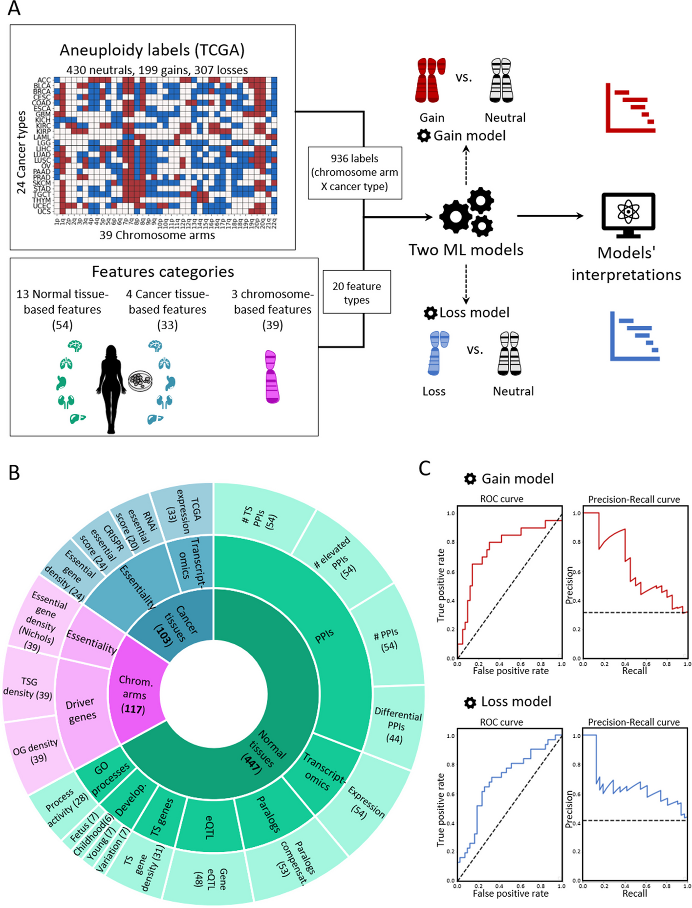
To create a supervised classification ML model that predicts the recurrence pattern of aneuploidy across cancer types, we built a large‐scale dataset consisting of labels and features per instance of chromosome-arm and cancer type. For each instance, the label indicated whether the chromosome-arm was recurrently gained, lost, or remained neutral in that cancer. Labels were determined according to Genomic Identification of Significant Targets in Cancer (GISTIC2.0) [24]. We focused on 24 cancer types for which transcriptomic data of normal tissues of origin was available from the Genotype-Tissue Expression Consortium (GTEx) ([25] (Methods). In total, 199 instances of chromosome-arm and cancer type were labeled as gained, 307 were labeled as lost, and 430 were labeled as neutral (Fig. 1A).

Fig. 1

A machine learning (ML) approach for predicting aneuploidy in cancer. A Schematic view of the ML model construction. Labels represent aneuploidy status of each chromosome arm in 24 cancer types (abbreviation of cancer types detailed in Additional file 2: Table S1), classified as gained (red, n = 199), lost (blue, n = 307), or neutral (white, n = 430). Features consist of 20 types of features pertaining to chromosome-arms, normal tissues and cancer tissues (see B). Two separate ML models were constructed to predict gained and lost chromosome-arms (gain model and loss model). Each model was analyzed to estimate the contribution of the features to the predicted outcome. B The features analyzed by the ML model. The inner layer shows feature categories: chromosome arms (purple), cancer tissues (primary tumors and CCLs, blue), and normal tissues (green). The middle layer shows the sub-categories of the features. Chromosome-arm features include essentiality and driver genes features. Cancer-tissue features include transcriptomics and essentiality features. Normal-tissue features include protein–protein interactions (PPIs), transcriptomics, paralogs, eQTL, tissue-specific (TS) genes, development, and GO processes features. The outer layer represents all 20 feature types that were analyzed by the model. Numbers in parentheses indicate the number of tissues, organs, or cell lines from which cancer and normal tissue features were derived, or the number of chromosome-arms from which chromosome-arm features were derived. C The performance of the ML models as evaluated by the area under the receiver-operating characteristic curve (auROC, left) and the precision recall curve (auPRC, right) using tenfold cross-validation. Gain model (gradient boosting): auROC = 74% and auPRC = 63% (expected 32%). Loss model (XGBoost): auROC = 70% and auPRC = 63% (expected 42%)

Next, we defined three categories of features (Fig. 1B; Methods). The first category, denoted ‘chromosome-arms’, contained features of chromosome-arms that are independent of cancer type. Chromosome-arm features included the density of OGs, the density of TSGs [6], and the density of essential genes [26] per chromosome-arm. The second category, denoted ‘cancer tissues’, contained features pertaining to chromosome-arms in primary tumors and CCLs. It included features pertaining to expression of genes in primary tumors and essentiality of genes in CCLs. Expression levels of genes in each chromosome-arm per cancer type were obtained from The Cancer Genome Atlas (TCGA, https://www.cancer.gov/tcga). Gene essentiality scores were obtained from the Cancer Dependency Map (DepMap) [27]. In total, this category included 103 omics-based readouts (Methods). The third category, denoted ‘normal tissues’, contained features pertaining to chromosome-arms in normal tissues from which cancer types originated (e.g., colon tissue was matched with colon adenocarcinoma, Additional file 2: Table S1). Features of normal tissues included expression levels of genes located on each chromosome-arm in the respective normal tissue, their tissue protein–protein interactions (PPIs) [28, 29], and their tissue-specific biological process activities [30]. It also included tissue-specific dosage relationships between paralogous genes, denoted ‘paralog compensation’ [31, 32]. In total, this category included 447 tissue-based properties (Methods). To enhance our understanding of cancer and tissue selectivity, feature values of cancer and normal tissues were transformed from absolute to relative; for example, instead of indicating the absolute expression level of a gene in a given normal tissue, the expression feature was set to the expression level of the gene in the given tissue relative to its expression levels in all tissues (Additional file 1: Fig. S1). Each chromosome-arm was then assigned with a feature value that was inferred from the values of its genes (Methods, Additional file 1: Fig. S2).

To fit the features dataset and the labels dataset, we further transformed the features dataset, such that each instance of chromosome-arm and cancer type was associated with features corresponding to the chromosome-arm, cancer type, and matching normal tissue (Methods). In total, the dataset included 20 types of features per chromosome-arm and cancer type: 3 in the chromosome-arm category, 4 in the cancer tissues category, and 13 in the normal tissues category (Fig. 1B). We assessed the similarity between every pair of features using Spearman correlation (Additional file 1: Fig. S3A). Most features did not correlate with each other (Additional file 1: Fig. S3B). Among the correlated feature pairs were PPI-related features and expression in normal adult and developing tissues features (Additional file 1: Fig. S3A). Lastly, we assessed the similarity between instances of chromosome-arm and cancer type by their feature values using principal component analysis (PCA) (Additional file 1: Fig. S3C). Instances did not cluster by their aneuploidy pattern (gain/loss/neutral), suggesting that a more complex model is needed to classify the different patterns.

With these labels and features of each chromosome-arm and cancer type, we set out to construct two separate ML models to predict chromosome-arm gain and loss patterns across cancer types (denoted as the ‘gain model’ and the ‘loss model’, respectively; Fig. 1A). Each model was trained and tested on data of gained (or lost) chromosome-arms versus neutral chromosome-arms. We employed five different ML methods (Methods) and assessed the performance of each method by using tenfold cross-validation and calculating average area under the receiver operating characteristic (auROC) and average area under the precision-recall curve (auPRC) (Additional file 1: Fig. S4A,B). Logistic regression showed similar results to a random prediction, with auROC of 54% for each model (Additional file 1: Fig. S4), indicating that the relationships between features and labels are non-linear. Decision tree methods that can capture such relationships [33, 34], including gradient boosting, XGBoost, and random forest, performed better than logistic regression and similarly to each other (Additional file 1: Fig. S4). Best performance in the gain model was achieved by gradient boosting method, with auROC of 74% and auPRC of 63% (expected: 32%) (Fig. 1C). Best performance in the loss model was achieved by XGBoost, with auROC of 70% and auPRC of 63% (expected: 42%) (Fig. 1C).

Revealing the top contributors to cancer aneuploidy patterns

The main purpose of our models was to identify the features that contribute the most to the recurrence patterns of aneuploidy observed in human cancer, which could illuminate the factors at play. To this aim, we used the SHAP (Shapley Additive exPlanations) algorithm [22, 23], which estimates the importance and relative contribution of each feature to the model’s decision and ranks them accordingly. We applied SHAP separately to the gain model and to the loss model (Methods).

In the gain model, the topmost features were TSG density and OG density (Fig. 2A,B). As expected, these features showed opposite directions: TSG density was low in gained chromosome-arms, whereas OG density was high, in line with previous observations [6, 7] (Fig. 2B). Importantly, this analysis revealed that the impact of TSGs on the gain model’s decision was twice larger than that of OGs (Fig. 2A), highlighting the importance of negative selection for shaping cancer aneuploidy patterns. The third most important feature was TCGA expression, which quantified the expression of arm-residing genes in the given cancer type relative to their expression in other cancers. Notably, expression levels were obtained only from samples where the chromosome-arm was not gained or lost (Methods). This analysis revealed that, across cancer types, chromosome-arms that tend to be gained exhibit higher expression of genes even in neutral cases, consistent with a previous recent study [8]. This confirms that the genes on gained chromosome-arms are preferentially important for the specific cancer types in which these gains are recurrent. Congruently, PPIs and normal tissue expression—features of normal tissues—were also among the ten top-contributing features (Fig. 2A). The estimated importance of all features in the gain model is shown in Additional file 1: Fig. S5A.

Fig. 2

Quantitative views into the ten topmost contributing features of the gain and loss models. Features are ordered from bottom to top by their increased average absolute contribution to the model, as calculated by SHAP. A The average absolute contribution of each feature to the gain model. The directionality of the feature (i.e., whether high feature values correspond to gain or neutral) is represented by an arrow. B A detailed view of the contribution of each feature to the gain model. Per feature, each dot represents the contribution per instance of a chromosome-arm and cancer type pair. The dots are spread based on whether they were classified as neutral (left) or gain (right) by the model. Instances are colored by the feature value (green-to-orange scale denotes low-to-high value). The order (height) of each feature is the same as in A. C Same as panel A for the loss model. D Same as panel B for the loss model. E The correlations between top contributing features and the frequencies of chromosome-arm gains and losses, as measured by Spearman correlation. P-values were adjusted for multiple hypothesis testing using Benjamini–Hochberg procedure. Negative correlation between TSG density and gain frequency (ρ = − 0.52, adjusted p = 0.006). Positive correlation between TSG density and loss frequency (ρ = 0.3, adjusted p = 0.17). Positive correlation between OG density and gain frequency (ρ = 0.25, adjusted p = 0.18). Negative correlation between OG density and loss frequency (ρ = − 0.47, adjusted p = 0.01). Positive correlation between TCGA expression and gain frequency (ρ = 0.29, adjusted p = 0.14). Negative correlation between TCGA expression and loss frequency (ρ = − 0.33, adjusted p = 0.12). Positive correlation between essential gene density and gain frequency (ρ = 0.16, adjusted p = 0.37). Negative correlation between essential gene density and loss frequency (ρ = − 0.1, adjusted p = 0.5)

The loss model shared the same top three features, yet with opposite directions and different ranks (Fig. 2C,D). OG density ranked first, was low in lost chromosome-arms, whereas TSG density ranked third, was high (Fig. 2D), in line with previous observations [6, 7]. In contrast to the gain model, in the loss model, the impact of OG density on the model’s decision was larger than that of TSG density, again in line with negative selection as an important force in cancer aneuploidy evolution. TCGA expression (computed from samples where the chromosome-arm was not lost or gained, see Methods) ranked second: chromosome-arms with highly-expressed genes tended not to be recurrently lost, in line with negative selection. Another top feature that showed opposite directions between the gain and loss model was essential gene density [26]. As expected, essential gene density was low in lost chromosome-arms, in line with negative selection against losing copies of essential genes [26, 27, 35]. The estimated importance of all features in the loss model is shown in Additional file 1: Fig. S5B.

To examine the direct relationships between high-ranking features and aneuploidy recurrence patterns, we assessed the correlations between these features and aneuploidy prevalence (Methods). In accordance with the SHAP analysis, the negative correlation between TSG density and chromosome-arm gain (ρ = − 0.52, adjusted p = 0.0006, Spearman correlation; Fig. 2E) was much stronger and more significant than the positive correlation between OG density and chromosome-arm gain (ρ = 0.25, adjusted p = 0.12, Spearman correlation; Fig. 2E). Similarly, the negative correlation between OG density and chromosome-arm loss (ρ = − 0.47, adjusted p = 0.003, Spearman correlation; Fig. 2E) was much stronger and more significant than the positive correlation between TSG density and chromosome-arm loss (ρ = 0.3, adjusted p = 0.067, Spearman correlation; Fig. 2E). TCGA expression and essential gene density were correlated with chromosome-arm gain, and anticorrelated with chromosome-arm loss, albeit to a lesser extent (Fig. 2E, Additional file 1: Fig. S6). Also showing positive correlations with gains and negative correlations with losses were features derived from expression levels in normal adult and developing tissues, certain PPI-related features, and additional essentiality features (Additional file 1: Fig. S6). However, these correlations were weaker than the correlations described above. Altogether, correlation analyses supported the relationships between top features of each model and aneuploidy patterns.

The robust impact of top contributors to cancer aneuploidy patterns

Next, we asked if the above results were sensitive to our model construction schemes. We first tested the robustness of the models to internal parameters used to generate the features (Methods). We therefore recreated features upon modifying internal parameters and repeated model construction and interpretation (Methods). We found that feature importance was robust to these changes (Additional file 1: Fig. S7, Additional file 3: Table S2). Second, we tested the robustness of the results upon tuning the hyperparameters of each model (Methods, Additional file 1: Fig. S8). The top contributing features of each model were retained following hyperparameter tuning, supporting their reliability (Additional file 1: Fig. S8C). We also checked whether the same top features would be recognized upon modeling one type of chromosome-arm event versus all other events. Applying the same approaches, we constructed two additional ML models. One model classified chromosome-arm gain versus no-gain (i.e., chromosome-arm loss or neutrality). Another model classified chromosome-arm loss versus no-loss (i.e., chromosome-arm gain or neutral). These additional models performed similarly to their respective models (Additional file 1: Fig. S9). SHAP analysis of the two additional models revealed that feature importance was very similar between these models and the original models, which compared gained and lost chromosome-arms only to neutral chromosome-arms (Additional file 1: Fig. S9).

We next tested whether the results were driven by a small subset of chromosome-arm and cancer type instances. For that, per model, we identified chromosome-arm and cancer type instances with the top contributions to the five topmost important features (Methods, Additional file 4: Table S3A,B, Additional file 5: Table S4A,B). Most instances contributed to at least one of these features, and none of the instances contributed to all five (Additional file 5: Table S4C). Next, we focused on chromosome-arm and cancer type instances that were top contributors to at least three of the five features (4.3% and 1.9% of the pairs in the gain and loss models, respectively). We tested their impact on the model by excluding them from the dataset and repeating the construction and interpretation of each model without them. The revised gain model retained its five topmost important features, though their ranking slightly changed (the third and fifth features switched). The revised loss model retained its four topmost important features (the fifth and seventh features switched) (Additional file 1: Fig. S10). This suggests that the general effect of the features was not driven by a small subset of instances.

Lastly, we expanded our analyses to address whole-chromosome gains and losses. For this, we updated the features dataset to refer to whole-chromosome and cancer type instances (Methods). For example, the feature TSG density was updated to refer to the entire chromosome. Likewise, we updated the aneuploidy status of whole-chromosome and cancer type instances using data from GISTIC (Methods). This resulted in a dataset of 78 whole-chromosome gains, 151 whole-chromosome loss, and 299 neutral cases. Next, we used these data to train a whole-chromosome gain (trisomy) model and a whole-chromosome loss (monosomy) model. Model training and assessment were similar to the chromosome-arm gain and loss models. Specifically, we employed five different ML methods and assessed their performance using fivefold cross-validation. Best performance for the trisomy model was achieved by random forest, with auROC of 69% and auPRC of 47% (expected 21%; Additional file 1: Fig. S11A). Best performance for the monosomy model was achieved by XGBoost, with auROC of 71% and auPRC of 59% (expected 34%; Additional file 1: Fig. S11D). Performances were somewhat weaker than the chromosome-arm models, in accordance with the training data being almost twofold smaller. Lastly, we interpreted each model using SHAP. In the trisomy model, the topmost feature was TSG density and its impact was over twofold larger than the impact of other features, similarly to the chromosome-arm gain model (Additional file 1: Fig. S11B,C). Other strong features of the chromosome-arm gain model, TCGA expression and OG density, ranked fifth and sixth, yet preserved their directionality. In the monosomy model, top features included OG density, TCGA expression, and paralogs compensation, fitting with the chromosome-arm loss model (Additional file 1: Fig. S11E,F). The feature TSG density was ranked eight, yet preserved its directionality, similarly to the remaining features. Altogether, these results suggest that negative selection is an important factor in shaping both chromosome-arm and whole-chromosome aneuploidy patterns.

Similar features shape aneuploidy patterns in human cancer cell lines and in human tumors

Next, we aimed to test whether similar features also shape aneuploidy patterns in CCLs. We collected data of aneuploidy patterns of all chromosome-arms in CCLs [36] and analyzed 10 cancer types with matched normal tissue data from GTEx [25] (Methods). Similar to the analysis of cancer tissues, we labeled each instance of chromosome-arm and CCL as recurrently gained (59 instances), recurrently lost (45 instances), or neutral (286 instances) and updated the features associated with cancer types according to the CCL data (Methods). We then applied the gain and loss ML models, which were trained on primary tumor data, to identify determinants of aneuploidy patterns of CCLs (Methods). The performance of the models was at least as good as for primary tumors (gain model: auROC = 83% and auPRC = 49% (expected 15%); loss model: auROC = 76% and auPRC = 45% (expected 11%), Fig. 3A). These results indicate that similar factors affect aneuploidy in cancers and in CCLs, consistent with the highly similar aneuploidy patterns observed in tumors and in CCLs [36, 37].

Fig. 3

Aneuploidy patterns in CCLs and primary tumors are shaped by similar features. A The ML scheme for analysis of aneuploidy patterns in CCLs. The gain and loss models that were trained on aneuploidy patterns in primary tumors were applied to aneuploidy patterns in CCLs. Performance was measured using tenfold cross-validation. Gain model (gradient boosting): auROC = 83%, auPRC = 49% (expected 15%). Loss model (XGBoost): auROC = 76%, auPRC = 45% (expected 11%). B The average absolute contribution of the ten topmost features to the gain model (see legend of Fig. 2A). The order and directionality of the features generally agree with the gain model in primary tumors. C A detailed view of the contribution of the ten topmost features to the gain model (see legend of Fig. 2B). D Same as B for the loss model. The order and directionality of the features generally agree with the loss model in primary tumors. E Same as panel C for the loss model. F The correlations between top contributing features and the frequencies of chromosome-arm gains and losses, as measured by Spearman correlation. p-values were adjusted for multiple hypothesis testing using Benjamini–Hochberg procedure. Negative correlation between TSG density and gain frequency (ρ = − 0.37, adjusted p = 0.04). Positive correlation between TSG density and loss frequency (ρ = 0.17, adjusted p = 0.32). Positive correlation between OG density and gain frequency (ρ = 0.44, adjusted p = 0.012). Negative correlation between OG density and loss frequency (ρ = − 0.28, adjusted p = 0.13). Positive correlation between CCL expression and gain frequency (ρ = 0.53, adjusted p = 0.002). Negative correlation between CCL expression and loss frequency (ρ = − 0.6, adjusted p = 0.0006). Positive correlation between essential gene density and gain frequency (ρ = 0.18, adjusted p = 0.33). Negative correlation between essential gene density and loss frequency (ρ = − 0.17, adjusted p = 0.32)

We next used SHAP to assess the contribution of each feature to each of the models. TSG density and OG density remained the top contributing features for the gain model. Consistent with our results in primary tumors, the contribution of TSG density was much stronger than that of OG density, confirming the role of negative selection (Fig. 3B,C). In the loss model, the ranking of top features was slightly different than in primary tumors (Fig. 3D). Expression in CCL was the top feature, such that recurrently lost chromosome-arms were associated with lower gene expression in neutral cases. OG density was one of the strongest contributing features for the loss model whereas TSG density had weaker contribution, again in line with negative selection playing an important role in shaping cancer aneuploidy landscapes (Fig. 3D,E). Certain features of normal tissues were also highly ranked. The contribution of essential gene density was also consistent with its impact in primary tumors (Fig. 3B,C).

As with the primary tumors, correlation analyses supported the contributions of the different features. CCL expression was highly correlated with chromosome-arm gain and anticorrelated with chromosome-arm loss (ρ = 0.54, adjusted p = 0.02, and ρ = − 0.6, adjusted p = 0.0006, respectively; Fig. 3F). Negative correlations were also observed between TSG density and gain frequency (ρ = − 0.37, adjusted p = 0.04, Spearman correlation; Fig. 3F) and between OG density and loss frequency (ρ = − 0.28, adjusted p = 0.1, Spearman correlation; Fig. 3F). Altogether, these results indicate that despite the continuous evolution of aneuploidy throughout CCL culture propagation [38], similar features drive aneuploidy recurrence patterns in primary tumors and in CCLs.

Chromosome 13q aneuploidy patterns are tissue-specific, and KLF5 is a driver of 13q gain in colorectal cancer

In human cancer, a chromosome-arm is either recurrently gained across cancer types or it is recurrently lost across cancer types, but rarely is a chromosome-arm both gained in some cancer types and lost in others [4, 5]. An intriguing exception is chr13q. Of all chromosome-arms, chr13q is the chromosome-arm with the highest density of tumor suppressor genes (Fig. 2E). It is therefore not surprising that chr13q is recurrently lost across multiple cancer types (with a median of 30% of the tumors losing one copy of 13q across cancer types) [4, 5]. Interestingly, however, chr13q is recurrently gained in human colorectal cancer (in 58% of the samples), suggesting that it can confer a selection advantage to colorectal cells in a tissue-specific manner. Indeed, when comparing colorectal tumors and colorectal cancer cell lines against all other cancer types, chr13q was the top differentially affected chromosome-arm (Fig. 4A,B). We therefore set out to study the basis for this unique tissue-specific aneuploidy pattern.

Fig. 4

KLF5 is a potential driver of chromosome 13q gain in human colorectal cancer. A Comparison of the prevalence of chromosome-arm aneuploidies in colorectal tumors against all other tumors (left) and colorectal cancer cell lines against all other cancer cell lines (right). On the right side are the aneuploidies that are more common in colorectal cancer, and on the left side are the ones that are less common in colorectal cancer. Chromosome-arm 13q (in red) is the top differential aneuploidy in colorectal cancer. B Comparison of the prevalence of 13q aneuploidy between colorectal tumors and all other tumors (left) and between colorectal cancer cell lines and all other cancer cell lines (right). ****, p < 0.0001 and ****, p < 0.0001; Chi-square test. C Genome-wide comparison of differentially essential genes between colorectal cancer cell lines (n = 85) and all other cancer cell lines (n = 1407). On the right side are the genes that are more essential in other cancer cell lines, and on the left side are those that are more essential in colorectal cancer, based on a genome-wide CRISPR/Cas9 knockout screens [39]. The x-axis presents the effect size (i.e., the differential response between colorectal cell lines and other cell lines), and the y-axis presents the significance of the difference (-log10(p-value)). KLF5 (in red) is the second most differentially essential gene in colorectal cancer cell lines. D Comparison of the sensitivity to CRISPR knockout of KLF5 between colorectal cancer cell lines (n = 59) and all other cancer cell lines (n = 1041). ****, p < 0.0001; two-tailed Mann–Whitney test. E Genome-wide comparison of differentially expressed genes between colorectal tumors (n = 434) and all other tumors (on the left, n = 11,060) and between colorectal cancer cell lines (n = 85) and all other cancer cell lines (on the right, n = 1407). On the right side are the genes that are over-expressed in colorectal cancer and on the left side are those that are over-expressed in other cell lines. KLF5 (in red) significantly over-expressed in colorectal cancer. F Comparison of KLF5 mRNA levels between colorectal tumors (n = 434) and all other tumors on the left (n = 11,060) and between colorectal cancer cell lines (n = 85) and all other cancer cell lines (on the right, n = 1407). ****, p < 0.0001; two-tailed Mann–Whitney test. G Correlation between KLF5 mRNA expression and the sensitivity to KLF5 knockdown, showing that higher KLF5 expression is associated with increased sensitivity to its RNAi-mediated knockdown. ρ = − 0.39, p = 0.01; Spearman correlation. H Comparison of KLF5 mRNA levels between DLD1-WT (without trisomy of chromosome 13) and DLD1-Ts13 (with trisomy of chromosome 13) colorectal cancer cells. **, p = 0.0025; one-sample t-test. I Representative images of DLD1-WT and DLD1-Ts13 cells treated with siRNA against KLF5. DLD1-Ts13 cells proliferated more slowly, as previously reported, but were more sensitive to the knockdown after accounting for their basal proliferation rate. Cell masking (shown in yellow) was performed using live cell imaging (IncuCyte) following 72 h of treatment. Scale bar 400µm. J Quantification of the relative response to KLF5 knockdown between DLD1-WT and DLD1-Ts13, as evaluated by quantifying cell viability in cells treated with siRNA against KLF5 versus a control siRNA for 72 h. n = 3 independent experiments. *, p = 0.0346; one-sided paired t-test

We performed a genome-wide comparison of differentially essential genes between colorectal cell lines and all other cell lines. The two top genes, which are much more essential in colorectal cancer cells than in other cancer types, were CTNNB1 and KLF5 (Fig. 4C). Of particular interest is KLF5, which is located on chr13q and colorectal cancer cell lines are significantly more sensitive to its knockout (Fig. 4D). KLF5 was reported to be tumor-suppressive in the context of several cancer types, such as breast and prostate [