1 Introduction

Neuroimaging covers various direct and indirect techniques used to visualize both the structure and the function of the nervous system. These methods include MR (Magnetic Resonance Imaging), CT (Computed Tomography), PET (Positron Emission Tomography), and EEG (electroencephalography). Among them, aside from being non-invasive, EEG retains some advantages over others such as high temporal resolution, easy accessibility, and low cost. Since EEG can capture brain activity in real-time in millisecond precision, it has become popular in neuroscience research, clinical diagnostics, and BCI (Brain-Computer Interface) systems. BCIs translate neural signals into commands for controlling external devices through software applications. In recent developments, researchers have delved into analyzing EEG patterns linked to particular finger movements. BCIs engineered to decipher these patterns offer the prospect of individuals operating external devices or interfaces solely through brain activity, eliminating the necessity for physical muscle movements. This advancement holds immense promise in crafting prosthetic hands capable of individual finger control, managing numerous devices, facilitating neurorehabilitation, and extending into applications within gaming and entertainment industries (Aricò et al., 2018). In the following subsections, after a literature review on both brain-computer interfaces and state-of-the-art finger movement classification studies, we mentioned our aim, our contributions to the literature, and the structural organization of this article, respectively.

1.1 Brain-computer interfaces

BCIs are computer-assisted systems that record the brain's electrical signals based on different brain monitoring techniques, analyze the signals on the interface, and convert them to specific commands to control external devices such as computers, wheelchairs, and prostheses without any physical movement (Belkacem et al., 2020). Consequently, BCI technology can help people suffering from various motor disabilities such as stroke patients to communicate with the outside, and indirectly perform motor function (Wolpaw et al., 2002). Among several different neuroimaging modalities, Electroencephalography (EEG) is widely used to capture brain activities. It is preferred for designing BCI systems due to the fact that EEG has many advantages such as its high temporal resolution, non-invasiveness, easy operation, relatively low cost, and portability (Vidal, 1977; Chen et al., 2015).

EEG-based BCI systems that manipulated motor imagery signals generated through the movements of large body parts such as hands, feet, and tongue have been proposed to control assistive devices throughout the past several decades (Pfurtscheller and Neuper, 2001; Alazrai et al., 2019; Degirmenci et al., 2023). However, such systems propose only limited control dimensions for prosthetic devices, thereby, the potential of utilizing these systems to control further complex assistive devices is restricted (Sciaraffa et al., 2022). In the last decade, numerous research studies have examined the decoding of movements of fine body parts to improve such systems (Alazrai et al., 2019).

The decoding of the movements performed by various fingers of a hand may increase the control dimensions of the EEG-based BCI systems. This, in turn, might provide subjects who utilize assistive devices to better carry out numerous skillful tasks. However, the decoding of finger movements (FM) within the same hand is considered as a demanding research area among motor imagery signal analysis studies (Alazrai et al., 2019). Employing and analyzing different kinds of feature extraction methods, feature selection methods, and classification algorithms play an important role in order to improve the efficiency of EEG-based BCI systems, which analyze FM and generate relevant commands from the recorded EEG data. In the literature, various feature extraction methods, feature reduction methods, and classification algorithms have been suggested for decoding FM. Different time-domain, frequency-domain, and spatial-domain EEG features have been calculated to predict FM in the past decade. The raw EEG time series (Kaya et al., 2018; Mwata-Velu et al., 2022; Zahra et al., 2022), different amplitude-based, and statistical-based EEG signal features (Degirmenci et al., 2024) were utilized to examine the effectiveness of the time domain. As for the spectral-domain features, different frequency-domain [Fourier transform (Kaya et al., 2018)] and time-frequency domain [Wavelet transform (Yahya et al., 2019), Short-time Fourier transform (Azizah et al., 2022), Empirical mode decomposition (Mwata-Velu et al., 2021)] representation algorithms and their various versions were investigated to classify FM. Common spatial pattern (Anam et al., 2019, 2020) and its different versions (Kato et al., 2020) are one of the most experimented methods for the analysis of spatial domain in FM classification. These different extracted features have been successfully classified using various machine learning algorithms. However, it is a challenging scientific task to determine and choose the most efficient combination of these methods. Providing optimal and relevant features is important for improving classifier performance (Narin et al., 2014; Degirmenci et al., 2023). Therefore, the implementation of effective feature extraction methods and feature reduction methods is essential for facilitating the following task of machine learning algorithms.

1.2 State of the art for finger movement classification

In the last decade, various signal processing and classification methods have been successful in FM classification (up to 91.70%) applied in the classification of EEG signals for FM tasks.

Kaya et al. (2018) conducted a Support Vector Machine (SVM) based classification study to classify the five FM of a hand. In their study, they used the data set they collected from a total of eight subjects who agreed to participate. They exploited the power of EEG subbands, Fourier Transform (FT) amplitudes, and EEG time series to represent 19-channel EEG signals as features. An average accuracy of 43.00% was obtained. Moreover, a subject-dependent classification study was also carried out and the performances of eight subjects were found to vary in the range of (20.00, 60.00%).

In Anam et al. (2019), the classification of five FM for the subject-dependent condition using the EEG signals of four subjects was aimed. To this purpose, the Common Spatial Pattern (CSP) based feature extraction process was performed and the Random Forest (RF) algorithm was executed. The classification performance was found to be 100% for training accuracy for each subject and the test accuracy performances ranged between 51.00 and 56.00%.

In 2022, Azizah et al. (2022) carried out a subject-dependent FM classification study. They performed channel selection based on One vs. Rest Common Spatial Pattern (CSP-OVR) and four out of 19 EEG channels were defined as relevant channels in their study. They extracted the spectrogram features from these selected channels. Their subject-dependent experimental results showed that the accuracy in classifications employing SVM ranged from 21.20 to 66.60%.

In the study conducted by Kato et al. (2020) in 2020, a multi-class CSP and Complex Fourier amplitudes-based feature extraction process was presented. They extracted features using 19 EEG channels for FM classification. According to their subject-dependent results, the training results of classifications carried out with the SVM algorithm were reported in the range of 23.90–58.30%.

Recently, deep learning approaches from machine learning methods have been the focus of attention by researchers in many different research areas such as disease detection from medical images (Narin and Isler, 2021), emotion recognition from biological signals (Ozdemir et al., 2021) and Electrocardiography (ECG) based arrhythmia detection (Degirmenci et al., 2022a) due to the fact that these architectures provide improved performance of classification. In addition, the main reason for this is that feature extraction and classification stages can be performed together in the hidden layers of deep learning structures. Considering these structures' benefits and advantages, deep learning approaches are also included for the classification of FM and motor imagery tasks in the literature.

In 2021, Mwata-Velu et al. (2021) performed a feature extraction process based on Empirical. Mode Decomposition (EMD) using four effective EEG channels which were selected from 19 EEG channels. They performed deep learning (BiLSTM) based subject-dependent classifications for the prediction of FM. Using EMD-based feature extraction and deep learning structure, training accuracy values in eight subjects were calculated in the range of 73.47- -98.69%, and test performances were calculated in the range of 66.00–76.13%.

In another study conducted in 2022, Mwata-Velu et al. (2022) worked on the classification of EEG time series with deep learning (EEGNet) structure. EEG signals of four subjects were used from a dataset that included EEG data of eight subjects, and at the same time, four out of 19 EEG channels were selected for their suggested study. In the subject-dependent analyses performed with four subjects, training successes were reported in the range of 80.10–91.70%.

In Anam et al. (2020), an FM classification study, a model that uses CSP algorithm-based feature extraction and Autonomous Deep Learning (ADL) based classification was proposed. They used 19-channel EEG signals from four subjects for their experimental process. With respect to the subject-dependent classifications, training performances ranged from 74.73 to 77.61%, and test performances ranged from 74.61 to 77.75%.

In another related paper Zahra et al. (2022), which was published recently in 2022, the performance of a Convolutional Neural Networks (CNN) was evaluated based on an original study design. In their model, EEG time series were combined with sliding window (Dietterich, 2002) and noise enhancement (Mitaim and Kosko, 1998) methods to extract the features. They obtained the features from 19-channel EEG signals of eight subjects. They conducted a subject-independent FM classification and achieved a training accuracy of 57.50%.

In their study conducted in 2022, Limbaga et al. (2022) carried out a CNN (EEGNet) based study for feature extraction and signal classification of five motor imagery classes of a hand. They reinforced their suggested model using a transfer learning approach through an EEG data set that includes 19-channel EEG signals of eight subjects. They reduced the EEG channel number to 14 and utilized the EEG signals of only four subjects. In addition to this data set, they recorded EEG signals from a subject while the subject imagined five different hand positions. According to their subject-independent evaluations, they achieved an accuracy of 51.74% success with the transfer learning model which is a reinforced model.

When the studies mentioned above that aimed to classify the motor imagery tasks of FM of a hand are examined, it was observed that the performances remained at relatively low rates in studies using all EEG channels and in subject-independent classification studies. The studies showed that the performances got higher with channel selection-based and subject-dependent classifications. The cause for the low level of performance in the classification of FM may be that the movements of the fingers on a hand are actually controlled from the same region of the motor cortex (Kaya et al., 2018). Kaya et al. (2018) investigated the event-related potential (ERP) curves of motor imagery tasks of other body limb movements together with motor imagery tasks of FM. They reported that the curves could not be clearly differentiated in the motor imagery tasks of FM. Therefore, there is a need to increase the classification performance by using effective feature extraction methods, feature selection methods, and classification algorithms for the classification of FM tasks.

1.3 The aim of the study

In 2007, an iterative signal decomposition technique, which is known as intrinsic time-scale decomposition, (ITD) was introduced to analyze nonlinear or non-stationary signals (Frei and Osorio, 2007). Recent studies have performed ITD-based approaches for the analysis of biomedical signals. ITD-based feature extraction processes were conducted in various EEG-based studies for different objectives such as epilepsy detection (Martis et al., 2013; Degirmenci and Akan, 2020), and attention deficit hyperactivity disorder (ADHD) recognition (Karabiber Cura et al., 2023). Considering its ability to discriminate different classes, we studied to explore whether ITD promises superior use, or not, in classifying other biomedical signals.

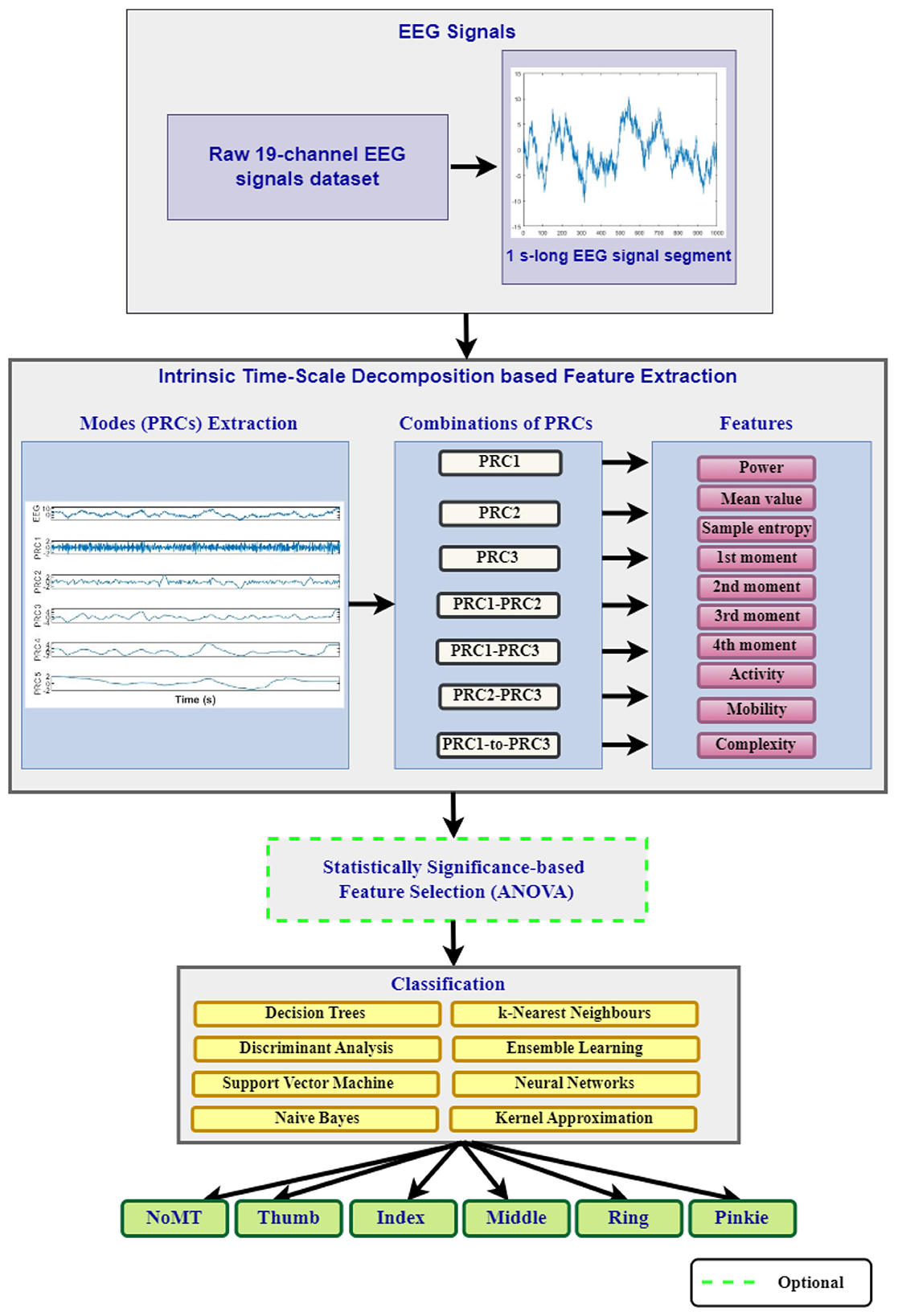
In this study, therefore, we suggest new praxis for the classification of FM tasks using ITD of EEG signals. The different modes that are defined as Proper Rotation Components (PRCs) and their combinations are acquired through ITD. Various features are evaluated using only modes and their combinations. In addition to the ITD-based feature extraction process, the effectiveness of statistically significance-based feature selection (ANOVA) is also investigated. The extracted ITD-based features are classified by eight different machine learning algorithms (Decision Tree, Discriminant Analysis, Naive Bayes, K-Nearest Neighbors, Support Vector Machine, Ensemble Learning, Neural Networks, and Kernel Approximation). Different performance evaluation metrics are employed for the accurate evaluation of the outputs of the suggested study.

1.4 Contributions

The novel contributions of this research study are summarized as follows:

• The classification of EEG signals of FM tasks is presented, using the ITD signal decomposition, and various feature extraction methods.

• Modes extracted by the ITD are utilized to evaluate several features, including Power, Mean, Sample Entropy, High-Frequency Moments (First Moment, Second Moment, Third Moment, Fourth Moment), and Hjorth Parameters (Activity, Mobility, Complexity).

• The first 3 modes (,, and ), and different combinations of them (,,, and ) are used for feature extraction and the effectiveness of only modes and their combinations are investigated with different machine learning algorithms, separately.

• The investigation of an appropriate and sustainable machine learning model for the proposed features to differentiate the FM tasks, and improve classification performance (success rate) as compared with the existing methods.

Finally, it must also be noted that this is the first study with a model that brings different combinations of PRCs extracted by ITD and various other features to classify FM tasks, to the best of our knowledge.

1.5 Paper organization

The rest of the paper is organized as follows: The EEG dataset used in this study, and EEG signal analysis methods are performed by the proposed ITD method which are ITD-based feature acquisition, statistical significance-based feature selection, classifier algorithms, and performance evaluation metrics are presented in Section 2. Experimental results are given in Section 3 and the results of the proposed approaches are discussed in Section 4. The outcomes of the study are summarized in Section 5.

2 Materials and methods

This study design mainly consists of five stages that are described in Isler (2009). These are EEG Data Acquisition, ITD-based Feature Extraction, Feature Reduction, Classification, and Performance Evaluation. The processes performed in each stage were delineated with details in the sub-headings. Out of these five stages/steps, the first four stages constitute the proposed classification model. Figure 1 shows the block diagram for the proposed model with its stages/steps.

Figure 1. The block diagram of the study.

2.1 EEG dataset description

In this study, the EEG dataset, which is a large electroencephalographic motor imagery dataset for EEG-based BCIs, presented by Kaya et al. (2018) is benefited. The dataset consists of motor imagery EEG signals that were recorded from 13 healthy subjects through 19 channels. 19 EEG electrodes together with two reference electrodes and the ground electrode were placed according to the international 10/20 EEG electrode placement system. The researchers reported that they recorded the EEG signals using an EEG-1200 JE-912A system. They performed an individual motor imagery experiment based on the movements of 10 different body limbs for four different BCI interaction paradigms. Among these planned paradigms, Paradigm #1-(CLA), which means classical left/right-hand motor imagery includes three imageries, and these are left and right-hand movements, and one passive mental imagery in which subjects remained neutral in no motor imagery. Paradigm #2-(HaLT), which means hand/leg/tongue motor imagery contains six tasks, and it is an extended version of the 3-state CLA paradigm with motor imagery tasks of right and left foot movement and tongue movement. Paradigm #3 (5F), which means 5-finger motor imagery includes FM imageries of the five-finger movement of a hand. During the tasks given for different fingers, subjects implemented the corresponding imageries invoking as flexion of the relevant finger up or down. Finger movement imageries were coded as follows: Thumb (Class 1), Index finger (Class 2), Middle finger (Class 3), Ring finger (Class 4), and Pinkie finger (Class 5). Paradigm #4 (NoMT), which means no imagery, visual stimuli only is the case in which no visual stimulus is presented to the subjects and they passively watch the computer screen. In this study, we aimed to carry out a 6-class classification using the 5F and NoMT paradigms. Whilst recording of EEG signals, the action signal remained on the screen for 1 s to implement the corresponding motor imageries. At the end of the given time, the task was not shown on the screen. Instead, the relevant task was interrupted for 1.5–2.5 s until the next task. In this dataset, two different sampling frequencies, 200 and 1,000 Hz, were set for experiments. EEG signals recorded with a 1000 Hz sampling frequency were extracted to be used in this study. In recording of EEG signals acquired at 1,000 Hz, a 0.53–100 Hz band-pass filter was applied to signals using hardware filters. In addition, a 50 Hz notch filter was applied to reduce the electrical grid interface. Before performing the feature extraction and the following steps, to have a balanced distribution among the classes and provide adjusted chance level (Galiotta et al., 2022), 100 samples of 1,000 Hz EEG signals for the 5F (five classes) and NoMT (one class) paradigms were studied for each class as the preprocessing stage. Hence, a total of 600 trials were performed for one subject. After obtaining the 5F and NoMT EEG signals for each subject, each EEG segment is decomposed to the finite number of PRCs by applying ITD.

2.2 Intrinsic time-scale decomposition (ITD)

ITD is introduced by Frei and Osorio for time-frequency-energy (TFE) analysis of signals with precision (Frei and Osorio, 2007). The ITD decomposes a signal into (i) a sum of PRCs, and (ii) a monotonic trend without the need for laborious and ineffective sifting or splines. It is an iterative decomposition algorithm for the analysis of nonlinear and non-stationary signals, decomposing the original signal into low-frequency, which is known as baseline signal (Lt), and high-frequency, which are known as proper rotation (Ht) components. ITD preserves precise temporal information (Frei and Osorio, 2007; Voznesensky and Kaplun, 2019; Degirmenci and Akan, 2020).

For the application of ITD, suppose there is an EEG signal Xt to be processed. To extract the low-frequency component (“baseline signal”) from the EEG signal, an operator ? is introduced and the remainder is the high-frequency component (“proper rotation”). Hence, the EEG signal Xt is defined as in Equation 1.

Xt=?Xt+(1-?)Xt=Lt+Ht    (1)

where the baseline signal is indicated as Lt = ?Xt, and the proper rotation component is indicated as Ht = (1 − ?)Xt. The extraction of baseline and proper rotation components are explained in detail with the following three steps (Frei and Osorio, 2007; Martis et al., 2013; Voznesensky and Kaplun, 2019):

• A real-valued signal is assumed as Xt, t ≥ 0 and τk, k = 1, 2, ⋯    denotes the its local extremes. Let the value of the signal at τk is denoted as X(τk) and the value of its baseline at τk is denoted as L(τk).

• We assume that Lt, and Ht have been defined over the interval [0, τk], and Xt is available for [0, τk + 2]. The baseline extraction operator, ? is provided as a piece-wise linear function on the interval (τk, τk + 1] between the two extrema as defined in Equations 2, 3.

Lt=Lk+(Lk+1-LkLk+2-Lk)(Xt-Xk), tϵ(τk,τk+1]    (2)

where

Lk+1=α[Xk+(τk+1-τkτk+2-τk)(Xk+2-Xk)]+(1-α)Xk+1,    (3)

and 0 < α < 1, is typically set with α=12. The baseline signal, Lt is constructed in this way to obtain the monotonicity of Xt between extrema. Hence, the baseline signal is reconstructed as a linearly transformed contraction of the original signal in conformity with Equations 2, 3.

• Once the baseline signal is defined, the residual or high-frequency component, PRC is computed as defined in Equation 4.

HXt=(1-?)Xt=Ht=Xt-Lt    (4)

Using the baseline Lt, and the high frequency Ht modes, the original signal Xt can be reconstructed using Equation 5.

Xt=LtD+∑j=0DHtj, j=0,⋯   ,D    (5)

where D denotes the number of PRCs that are provided during ITD processing.

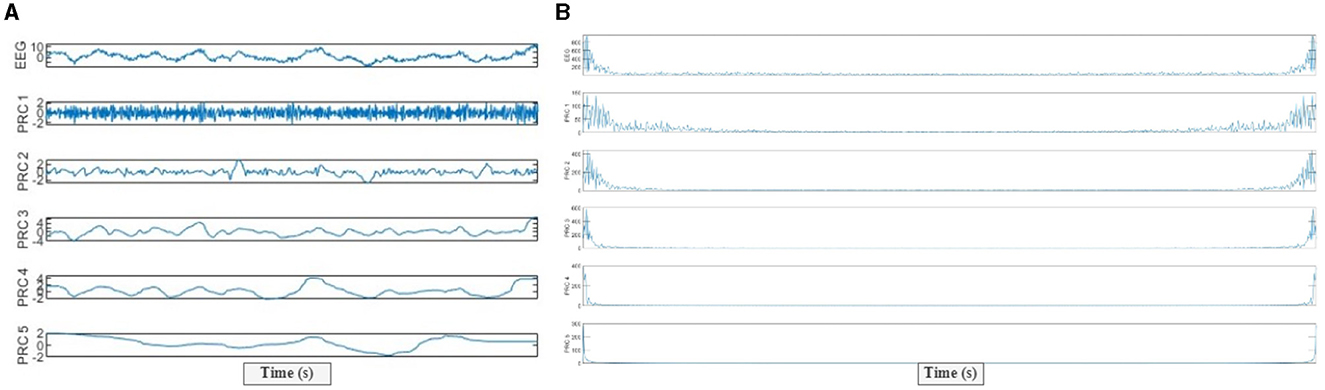
An exemplary motor imagery EEG signal decomposition process conducted through the ITD algorithm is given in Figure 2A. To decide which of the separate PRCs to work with, the PRCs were examined in the frequency domain and their energy spectrums were computed. In Figure 2B, a case of energy spectrums of PRCs, decomposed into an EEG signal is provided. Figure 2B shows that the first PRC (i.e., PRC1) has the highest frequency content, while the fifth PRC (i.e., PRC5) exhibits the lowest frequency content. Hence, we selected the first three PRCs and their different combinations for our suggested feature extraction process due to the fact that they include high-frequency contents that best represent the signal characteristic of the original EEG. Various feature extraction methods are implemented to the determined high-frequency PRCs (Ht), which are decomposed through ITD. In our study design, seven different sets of high-frequency PRCs which are only PRC1, PRC2, and PRC3, and their different combinations [PRC1–PRC2, PRC1–PRC3, PRC2–PRC3, and PRC1–PRC2–PRC3 (denoted as PRC1-to-3)] are acquired and utilized to evaluate 10 features.

Figure 2. (A) PRCs extracted by the intrinsic time-scale decomposition (ITD) from a 1-s segment of EEG signals, (B) Energies of each PRCs (the first five modes are given as examples).

2.3 ITD features

Following the extraction of low-frequency baseline signal and high-frequency PRCs by running the ITD algorithm, EEG signal properties including the power, mean value, sample entropy, high-frequency moments (first moment, second moment, third moment, and fourth moment), and Hjorth parameters (activity, mobility, and complexity) were computed from various combinations of PRCs. Their details are described below:

• The mean value was calculated based on time-domain information for 3 PRCs. It is defined as in Equation 6.

μ=1N∑n=0N-1X[n]    (6)

where PRCs are denoted as X[k], the mean value is denoted as μ and the size of PRCs is described as N.

• The total power of PRCs was obtained using the spectrum of signals. The spectrum of PRCs was evaluated by implementing the periodogram method, which allows for analysis of the frequency content of a signal (Iscan et al., 2011; Karabiber Cura et al., 2023). From definitions of k-th frequency (Equation 7) and power power spectral desity estimation of the k-th frequency component (Equation 8), the total power is defined as in Equation 9 (Iscan et al., 2011):

wk=2πNk,k=0,1,⋯   ,N-1    (7) S(wk)=1N|X(wk)|2    (8) ST=∑k=0N-1S(wk)    (9)

where S(wk) indicates the power spectral density of the signal provided by the periodogram method, X(wk) indicates the discrete Fourier transform of the PRC x[n], and ST is the total power of PRCs. N shown in Equations 8, 9, refers to the size of the corresponding signal.

• The higher order spectral moments (1st, 2nd, 3rd, and 4th) were computed using the spectrum of signals like total power. These moments are defined as in Equations 10–13, respectively (Degirmenci et al., 2018):

M1=∑k=0N-1(wk)1S(wk)    (10) M2=∑k=0N-1(wk)2S(wk)    (11) M3=∑k=0N-1(wk)3S(wk)    (12) M4=∑k=0N-1(wk)4S(wk)    (13)

Here, M1, M2, M3, and M4 represent the 1st, 2nd, 3rd, and 4th higher order spectral moments of the corresponding PRCs, respectively.

• Hjorth parameters were introduced by Hjorth (1970) in 1970, and these are time-domain statistical features used in signal processing. These parameters include the Activity parameter (Ax), Mobility parameter (Mx), and Complexity parameter (Cx) of the signal. In the following mathematical equations for Activity, Mobility, and Complexity parameters, y(n) indicates the auto-correlation function of one PRC after the ITD application. y[n] = [y1, y2, ⋯   , yN], and N indicates the length of the signal.

Activity parameter, defines the power of vibration signal and can be evaluated using the variance of signal amplitude. It is formulated in Equation 14 (Hjorth, 1970; Yu and Fang, 2022):

Ax=(y(n))=σy2    (14)

where σy denotes the standard deviation of y(n) and it can be described with the Equation 15.

σy=1N-1∑n=1N[y(n)-μ]2    (15)

Here, the mean value of the signal is represented with μ.

Mobility parameter describes the ratio of standard deviations of first-order derivatives, and it can be evaluated using the slope of the signal. It is defined as in Equation 16.

Mx=σy′2σy2=σy′σy    (16)

where σy′ indicates the first-order standard deviation of signals.

Complexity parameter denotes the similarity of signal to sinusoidal signal and it is expressed as the ratio between the mobility of the first derivative of the EEG signal and the mobility of the EEG signal itself (Hjorth, 1970; Yu and Fang, 2022). The mathematical expression of complexity parameters is given in Equation 17.

Cx=Mx(y′(t))Mx(y(t))=Mx(dy(t)dt)Mx(y(t))=σy″2σy′2σy′2σy2    (17)

Here, the second-order standard deviation of signal y(t) is expressed as σy″.

• The sample entropy indicates a time series complexity measure that represents the probability of a system generating new patterns. It can be defined as the embedding theory that utilizes the time series directly instead of probability values. The original time series is defined as Lt(i), i = 1, 2, ⋯   , N. The new vector sequences which each of size m, u(1) by u(N − m + 1) are created, and expressed as u(i) = (Higuchi, 1988; Martis et al., 2013). The defined length m indicates the embedding dimension. The distance d[u(i), u(j)] between vectors u(i), and u(j) is described in Equation 18 (Higuchi, 1988):

d(u(i),