1 Introduction

Recently, the advent of genetically encoded optical sensors has significantly enhanced the opportunities of experimental neurophysiology. Despite their wide use in various synapses (Borghuis et al., 2013; Taschenberger et al., 2016; Sakamoto et al., 2018; Pichler and Lagnado, 2019; Özçete and Moser, 2021; Vevea et al., 2021; Mendonça et al., 2022), relatively little attention has been given to potential interference with physiological neurotransmitter signaling and the established electrophysiological measurements.

Currently available genetically encoded glutamate indicators (GEGIs) are based either on AMPA receptors (AMPAR), like EOS (Namiki et al., 2007), or on bacterial glutamate binding proteins, such as GluSnFR, SuperGluSnFR (Hires et al., 2008), FLIPE (Okumoto et al., 2005), iGluSnFR (Marvin et al., 2013) and variants (Helassa et al., 2018; Marvin et al., 2018). These optical methods allow highly resolved measurement of synaptic glutamate and its spatial profile in near-physiological conditions, but are limited in the temporal domain by their slow decay kinetics, and constraints set by photobleaching and lateral tissue movement (Dürst et al., 2019).

Yet they have helped overcome several problems of previously used techniques such as microdialysis (Benveniste et al., 1984) or enzymatically coupled amperometry (Hu et al., 1994), which have usually sampled over time frames of at least a few hundred milliseconds, too long to measure millisecond changes during synaptic activity.

On short time scales, presynaptic function is typically evaluated using electrophysiological measurements: either by presynaptic capacitance recordings, which measure the change in presynaptic membrane surface area during synaptic vesicle (SV) exocytosis (and endocytosis), or postsynaptic recordings, in which the presynaptic activity is filtered through the response characteristics of the postsynaptic receptors.

Both iGluSnFR and electrophysiological measurements give quantitative insights into the dynamics of glutamate release. Recently, Armbruster et al. (2020) indicated that iGluSnFR expression in synaptic or perisynaptic membranes can alter physiological glutamate signaling. They used Monte-Carlo simulations and recordings of astrocyte glutamate transporter currents in order to study the influence of iGluSnFR on glutamate dynamics by glutamate buffering. Their results suggest that iGluSnFR reduces the amount of free glutamate in and around the synaptic cleft, dependent on iGluSnFR expression levels and distance from the release site. Since the utility of GEGIs for the study of synaptic physiology relies on GEGIs or the expression system not interfering with physiological glutamate signaling, further experimental exploration of this proposed mechanism is warranted.

In the present study, we express iGluSnFR in the presynaptic membrane of auditory nerve fibers (ANFs) in the anteroventral cochlear nucleus (AVCN) to further investigate the potential influence on physiological glutamate signaling. Spherical and globular bushy cells (BCs) in the AVCN receive few large axo-somatic inputs from spiral ganglion neurons (SGNs) (Brawer and Morest, 1975; Tolbert and Morest, 1982; Ryugo and Sento, 1991; Liberman, 1993; Spirou et al., 2005; Cao and Oertel, 2010). These large calyceal terminals are called endbulbs of Held (for the ANF—spherical BC synapse, Held, 1893; Ryugo and Fekete, 1982) or modified endbulbs of Held (ANF—globular BC, Rouiller et al., 1986), and are responsible for eliciting large, precisely timed, mainly AMPAR-mediated (Wang et al., 1998; Gardner et al., 2001; Schmid et al., 2001; Sugden et al., 2002; Cao and Oertel, 2010; Antunes et al., 2020), EPSCs in the postsynaptic BC soma. Endbulbs of Held are a well-studied model synapses, where a wealth of details about the presynaptic function is known, mostly through the availability of highly resolved electrophysiological data (Wang and Manis, 2008; Yang and Xu-Friedman, 2008, 2009, 2012; Cao and Oertel, 2010; Lin et al., 2011; Butola et al., 2017).

2 Methods and materials 2.1 Animal handling

We expressed iGluSnFR in SGNs of C57Bl/6J mice via viral vector injection into the neonatal cochlea as described previously (Özçete and Moser, 2021). Electrophysiological and imaging data was recorded from injected mice and their uninjected littermates of either sex from postnatal day 16 to 25 (P16 to P25). All experiments were performed in accordance to German national animal guidelines and were approved by the animal welfare office of the state of Lower Saxony as well as the local animal welfare office at the University Medical Center Göttingen (permit number: 17-2394). The AAV carrying the plasmid coding for iGluSnFR under the human synapsin promoter (pAAV.hSyn.iGluSnFR.WPRE.SV40) was a generous gift from Laren Looger (Addgene viral prep # 98929-AAV9) or produced in our own laboratory. Vector injections were performed as described before (Jung et al., 2015). In brief, P5 to P7 wildtype mice were anesthetized with isoflurane and the body temperature was kept at 37°C with a temperature plate and a rectal temperature probe. Under local anesthesia with xylocaine, the right ear was accessed through a dorsal incision and the round window exposed. 1–1.5 μL of suspended viral particles (titer ≥1013 vg/ml) were injected through the round window into the scala tympani through a quartz capillary. After the surgery, the incision wound was sutured and buprenorphine (0.1 mg/kg body weight) was applied for pain relief. The recovery status of the mice was monitored daily. Before and after the surgery, animals were kept with their mother and littermates until weaning (ca. P21) in a 12 h light/dark cycle, with access to food and water ad libitum.

2.2 Tissue preparation

Brainstem slices were prepared as described previously (Butola et al., 2017). Briefly, mice were decapitated and the brain was rapidly removed and placed into ice-cold cutting solution, containing in mM: 50 NaCl, 120 sucrose, 20 glucose, 0.2 CaCl2, 6 MgCl2, 0.7 sodium ascorbate, 2 sodium pyruvate, 3 myo-inositol, 3 sodium l-lactate, 26 NaHCO3, 1.25 NaH2PO4textrmcdotH2O, 2.5 KCl with pH adjusted to 7.4 and an osmolarity of around 320 mOsm/l. Meninges were removed with a forceps and hemispheres were separated using a blade. After removing extraneous tissue, the brain stem was glued to a block with cyanoacrylate glue (Loctite 401, Henkel) and 150 μm thick parasaggital slices containing the cochlear nucleus were cut with a Leica VT1200 vibratome (Wetzlar, Germany) for imaging and electrophysiology. After cutting, slices were allowed to equilibrate at 35°C for 30 min in artificial cerebrospinal fluid (aCSF) and kept at room temperature until used for electrophysiological recordings. The aCSF used for incubation contained (in mM: 125 NaCl, 13 Glucose, 1.5 CaCl2, 1 MgCl2, 0.7 sodium ascorbate, 2 sodium pyruvate, 3 myo-inositol, 3 sodium l-lactate, 26 NaHCO3, 1.25 NaH2PO4textrmcdotH2O, 2.5 KCl with pH adjusted to 7.4 and an osmolarity of around 310 mOsm/l. Slices were successively transferred to a recording chamber and continuously superfused with saline solution containing (in mM) 125 NaCl, 13 Glucose, 2 or 4 CaCl2, 1 MgCl2, 0.7 sodium ascorbate, 2 sodium pyruvate, 3 myo-inositol, 3 sodium l-lactate, 26 NaHCO3, 1.25 NaH2PO4 · H2O, 2.5 KCl with an osmolarity of around 310 mOsm/l and a pH of 7.4. The chamber was mounted on a Axioskop 2 FS plus upright microscope (Zeiss, Oberkochen, Germany) and the sample was illuminated with differential interference contrast (DIC) optics through a 40 × /0.8 NA water-immersion objective (Achroplan, Zeiss, Oberkochen, Germany).

2.3 Electrophysiology

Electrophysiological recordings were obtained from BCs in the anteroventral cochlear nucleus, which was localized in its characteristic position in respect to cerebellum, the cochlear nerve and the dorsal cochlear nucleus. Whole-cell patch clamp recordings of cells in the cochlear nucleus were performed with 2 – 4 MΩ pipettes pulled from borosilicate glass (GB150F, 0.86 × 1.50 × 80mm; Science Products, Hofheim, Germany) with a P-87 micropipette puller (Sutter Instruments Co., Novato, CA, USA, which were filled with intracellular solution, containing (in mM) 120 potassium gluconate, 10 HEPES, 8 EGTA, 10 sodium phosphocreatine, 4 ATP–Mg, 0.3 GTP–Na, 10 NaCl, 4.5 MgCl2, 0.001 QX-314 and 1 Alexa-596 anatomical dye, with an osmolarity of around 300 mOsm/l and a pH of 7.3 (adjusted with KOH). ANFs project onto multiple primary cells types in the cochlear nucleus (Brawer et al., 1974). In the AVCN, the two most prominent cell types are BCs and stellate cells (Brawer et al., 1974; Brawer and Morest, 1975). These cells are distinct in morphology and physiology (Wu and Oertel, 1984) and can be differentiated in a number of ways. As identified in Golgi stains, BCs have one axon and a singular dendrite, while stellate cells have three or more protrusions (Brawer et al., 1974; Wu and Oertel, 1984). Physiologically, stellate cells have a linear current-voltage relationship around the resting membrane potential and react to sustained depolarizing current injections with regularly firing action potentials (Wu and Oertel, 1984). Voltage-clamped, they react to stimulation of the afferent ANF with relatively broad and small eEPSCs (Wu and Oertel, 1984) and in response to spontaneous release, they show infrequent, small, and broad mEPSCs (Lu et al., 2007). In contrast, the input resistance of BCs markedly decreases for depolarizing current injections and they show large and fast eEPSCs (Wu and Oertel, 1984) and mEPSCs (Lu et al., 2007). Additionally, Chanda and Xu-Friedman (2010) showed that stellate cells and BCs differ in response to two consecutive ANF stimulation and the ratio of the eEPSCs in response to two pulses, 10 ms apart, the 10 ms paired-pulse ratio (PPR), can be used to divide BCs and stellate cells in two non-overlapping clusters, as eEPSCs in stellate cell facilitate while they depress in BC. To obtain a uniform cell population and because QX-314 interferes with normal action potential generation and thus prevents the easiest and most reliable identification method in current-clamp, BCs were identified in three ways: (i) through the frequency, size and decay time of their mEPSCs, once stimulation had been established through (ii) the response to consecutive stimulations and the width and duration of the eEPSCs and after finishing experiments and carefully retracting the patch pipette through (iii) morphological identification with fluorescence imaging Alexa-568 using a 585 nm LED (p100, CoolLED, Andover, UK) and a standard mCherry filter cube (Semrock, Rochester, NY, USA).

Data was recorded with a HEKA EPC 10 amplifier (HEKA Elektronik, Lambrecht/ Pfalz, Germany). Recordings were digitized at 40 kHz and low-pass filtered at 7.3 kHz. A liquid junction potential of 12 mV was corrected on-line. For confirmed BCs, EPSCs were evoked using monopolar direct current injections (5 – 20 μA), generated with a linear stimulus isolator (WPI Stimulus Isolator A365, World Precision Instruments, Sarasota, FL, USA). This was achieved by placing an electrode in a saline-filled patch pipette in a distance of 15 – 30 μm from the cell and during continuous monitoring of the membrane current, increasing the injected current until a single eEPSC could be triggered. The input was confirmed to be indeed monosynaptic by reducing the injected current until any further reduction lead to a complete failure of eEPSC generation. If successfully confirmed, the input was stimulated with breaks in between trains of stimuli of 30 s.All recordings were performed at -70mV (corrected for the liquid junction potential) unless stated differently. mEPSC recordings were performed in 2 mM [Ca2+]e. eEPSCs were recorded in either 2 or 4 mM [Ca2+]e and following drugs were added to the bath solution exclusively for eEPSC recordings: 10 μM bicuculline methchloride and 2 μM strychnine hydrochloride in order to block inhibitory GABAergic and glycinergic currents, respectively, and 1 mM sodium kynurenate to prevent AMPAR saturation and desensitization.

2.4 Glutamate imaging

iGluSnFR was excited using a 470 nm LED (p100, CoolLED, Andover, UK) and glutamate signals were recorded using a sCMOS digital camera (OrcaFlash 4.0, Hamamatsu, Hamamatsu City, Japan) mounted to the microscope using astandard GFP filter cube (Semrock, Rochester, NY, USA). Optimal LED intensity was chosen empirically as the minimal intensity at which a response could be seen reliably, usually at 0.5 – 1 mW/mm2.

Acquisition was triggered with a 5 mV pulse controlled by the patch clamp amplifier and synchronized to the current injections. For each stimulation, 1,200 ms of iGluSnFR signal were recorded after the first stimulation. The prior 1,300 ms were universally collected as background image.

2.5 Immunohistochemistry

For immunohistochemical analysis, different routes were chosen with respect to the tissue at hand. For cochleae, blocks containing the entire inner ear were obtained from the same animals used for in-vitro electrophysiology and glutamate imaging and immediately fixated using 4% (v/v) formaldehyde (FA) [diluted from 37% stock with phosphate-buffered saline (PBS)] for 20 min and washed with PBS. Cochleae were cryosectioned after a 0.12 mM EDTA decalcification. For brainstem, slices were fixed after electrophysiological experiments with 3% para-formaldehyde (PFA) for 15 min and washed with PBS. Sections were incubated for 1 h in goat serum dilution buffer (16% normal goat serum, 450 mM NaCl, 0.6% Triton X-100, 20 mM phosphate buffer, pH 7.4), primary antibodies were applied overnight at 4°C, after which secondary antibodies were applied for 1 h at room temperature. The following antibodies were used for the staining of the cochleae: chicken anti-GFP (Abcam, 1:500), rabbit anti-calretinin (Synaptic Systems, 1:2,000) and guinea pig anti-parvalbumin (Synaptic Systems, 1:300) and secondary AlexaFluor-labeled antibodies (goat anti-chicken 488 IgG, Thermo Fisher Scientific, 1:200; goat anti-guinea pig 568 IgG, Thermo Fisher Scientific, 1:200; goat anti-rabbit 633 IgG, Thermo Fisher Scientific, 1:200) For brainstem sections, primary antibodies used were an Alexa-488 labeled rabbit anti-GFP (Thermo Fisher Scientific, 1:400) and guinea pig anti-bassoon (Synaptic Systems, 1:500) and secondary goat anti-guinea pig 633 IgG (Thermo Fisher Scientific, 1:200). Confocal sections were acquired with a laser-scanning confocal microscope (Leica LSM780, Leica, Wetzlar, Germany), equipped with a 488 nm, a 561 nm and a 631 nm laser through a 63 × /1.4 NA oil-immersion objective (Plan-Apochromat, Zeiss, Oberkochen, Germany). Pin hole size was set to 1.0 airy units.

2.6 Data analysis

All electrophysiological data was exported from .dat files using Igor Pro 6.3.2 software (Wavemetrics, Lake Oswego, OR) running an instance of Patcher' Power Tools (Department of Membrane Biophysics, Max Planck Institute for Multidisciplinary Science, Göttingen, Germany) to .ibw files.

For the analysis of mEPSCs, Igor Pro 6.3.2 software together with a customized instance of the Quanta Analysis procedure (Mosharov, 2008) were used. Data was smoothened with a binomial filter at a corner frequency of 8 kHz. Recording quality and low-frequency noise level were sufficiently good to preclude further notch filtering. Peaks were automatically detected in an additionally filtered trace (1-dimensional Gaussian filter with a corner frequency of 2 kHz) and an additionally filtered derivative trace (1-dimensional Gaussian filter, corner frequency of 4 kHz), using a 5σ cutoff and manually inspected to ensure correct classifications as event. The rising phase was fit with a simple affine function, while the decay phase was fit with a single exponential. For further analysis and illustration, the median fit parameters as well as an averaged wave was extracted per cell. Other electrophysiological data was analyzed using a custom-written python script using the Neo wrapper for .ibw files (Garcia et al., 2014).

2.6.1 Deconvolution analysis

For some parts of the analysis, timeseries data derived from glutamate imaging was subject to deconvolution analysis. Since different approaches have been used in imaging and electrophysiological studies, we applied two different methods to deconvolve iGluSnFR signal.

The first approach, a Wiener deconvolution algorithm based on the discrete Fourier transform and its inversion, has been used in electrophysiological studies in end-plate currents at the neuromuscular junction (Van der Kloot, 1988) and for image analysis of iGluSnFR data (Taschenberger et al., 2016; James et al., 2019). The iGluSnFR signal s(t) was modeled as

s(t)=h(t)*x(t)+n(t),    (1)

where h(t) is the impulse response of the linear time-invariant system, x(t) the unknown signal, n(t) the additional noise and h(t)*x(t):=∫−∞∞h(t′)x(t−t′)dt′ is the convolution of h(t) and x(t). The Wiener deconvolution based on the model in Equation 1 gives an estimate of X(f), the Fourier transform of x(t), as

X(f)=S(f)H*(f)H(f)H*(f)+1SNR,    (2)

where S(f) is the transform of s(t), H(f) is the Fourier transform of h(t), H*(f) the complex conjugate of H(f) and SNR the signal-to-noise ratio. The SNR was estimated as the squared quotient of maximum response amplitude and root-mean-square noise of the baseline of the recording. The deconvolution algorithm based on Equation 2 was implemented in a custom-written python script using the fast Fourier transform algorithm and matrix algebra tools provided in the numpy package.

A second method has been described for the analysis of end-plate currents at the neuromuscular junction (Cohen et al., 1981) and has recently been adapted to derive pool parameters from timeseries data generated by EOS imaging (Sakamoto et al., 2018). Here, a derivation for glutamate imaging data is presented.

Suppose that the glutamate content in one SV is able to induce a response of n iGluSnFR molecules, leading a change in fluorescence of s0: = n·g0, where g0 is the unitary response. Between t0′ and t1′, in an interval δt′=t1′-t0′, SVs are released as a function of time x(t0′)·δt′, each leading to a change in fluorescence of s0. Suppose further that the fluorescence is constant for each iGluSnFR copy over the course of δt′ and that iGluSnFR switch to a state of lower fluorescence stochastically and the time each iGluSnFR stays in the activated state is distributed exponentially, assuming monoexponential unbinding kinetics (Helassa et al., 2018).

The average iGluSnFR response δs during δt′ is thus given by

δs(t′)=x(t′)·δt′·s0·exp(-t-t′τ),    (3)

where τ is the average time an iGluSnFR copy stays in an activated state. Integrating Equation 3 over all intervals yields

s(t)=s0·∫0tx(t′)·exp(−t−t′τ)dt′.    (4)

Differentiation of Equation 4 with respect to t as a parameter and integration limit yields

ds(t)dt=s0·x(t)−s0τ∫0tx(t′)·exp(−t−t′τ)dt′.    (5)

Substituting Equation 4 in Equation 5 reduces the expression to

ds(t)dt=s0·x(t)-s(t)τ.    (6)

Thus, the signal can be deconvolved by

s0·x(t)=ds(t)dt+s(t)τ.    (7)

For computation of Equation 7, the derivative ds(t)/dt(t′) was approximated as s(t′+Δt)−s(t′)/Δt. The error associated with r: = s0·x(t) was approximated by

σr=2σsΔt-σsτ-s(t)τ2στ.

In electrophysiological recordings, quantal currents (either in the sense of unitary ion channel currents or currents induced by one released SV) are usually accessible through noise analysis. For glutamate imaging data, this approach has been successful in low-noise recordings of hippocampal cultures (Sakamoto et al., 2018). If the amplitude of the signal induced by one SV is not known, this approach still gives relevant information of relative release rates, e.g. over the course of multiple stimulations.

During stimulations, τ can be estimated as the time constant of a single exponential fit through the decay phase of the signal. This estimation is an upper bound for τ, as it assumes that all SVs are released and all iGluSnFR copies are activated simultaneously.

For practical calculations, this method was implemented in python, using a numerical approximation to the derivative provided in the numpy package.

2.6.2 Statistical analysis

If not indicated differently, means are given ± standard error of the mean. For derived quantities, standard errors were calculated taking gaussian error propagation into account. Statistical analysis was performed with consideration of clustering effects introduced by repeated measurements of the same cell, when appropriate. If clustering was not relevant to the statistical analysis, statistical significance was determined by the Wilcoxon rank sum test. When clustering had to be taken into account, condition effects were estimated using a mixed effects model with a random cell-specific intercept (for discussions of different approaches to clustered data in neuroscience research see Galbraith et al., 2010; Yu et al., 2022). When given, p values are presented as an exact number, except if smaller than 0.001 (for a discussion see Wasserstein and Lazar, 2016). If effects are described as “statistically significant”, a canonical significance level of α = 0.05 was assumed. When a number m of multiple comparisons were performed, Bonferroni-adjusted significance levels α* = α/m are noted.

Statistical analysis was performed using custom-written python scripts, using implementations in the statsmodels and scipy packages.

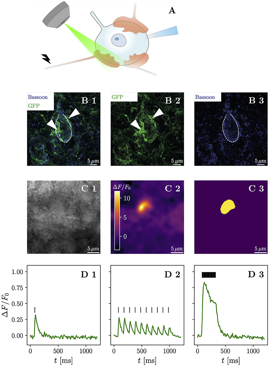
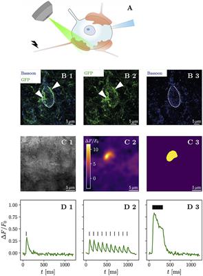
3 Results 3.1 iGluSnFR expressed in SGNs reports glutamate release at the endbulb of Held

To measure glutamate release at the endbulb terminals (for a schematic drawing see Figure 1A) of ANFs, we introduced iGluSnFR into SGNs. To our knowledge, no previous studies have used genetically encoded activity indicators in the cochlear nucleus. Here, a viral vector, adeno-associated virus (AAV) 2/9 carrying iGluSnFR under the control of the human synapsin promoter, was injected into the cochlea, targeting SGN cell bodies located in the modiolus. Injections through the round window are established in intracochlear pharmaco- and gene therapy (e.g., Chen et al., 2003; Akil et al., 2012; Askew et al., 2015; Jung et al., 2015) and have been used to deliver small compounds like calcium dyes (Chanda et al., 2011; Zhuang et al., 2020), optogenetic tools, including iGluSnFR (e.g., Keppeler et al., 2018; Özçete and Moser, 2021), to SGN cell bodies and axons projecting onto inner hair cells. Importantly, in the studies where auditory function was tested including Özçete and Moser (2021) which used the same expression strategy as we used here and tested auditory function with auditory brainstem recordings, no indication of impairment was found in the treated mice.

Figure 1. High-frequency stimulation of iGluSnFR-expressing presynaptic terminals allows discrimination of contiguous loci of glutamate release. (A) Shows a schematic drawing of the anatomical characteristics of the endbulb of Held and the typical postsynaptic patch-clamp recording situation with simultaneous iGluSnFR imaging during affarent fiber stimulation. Usually, between 3 and 5 large calyceal axosomatic synapses are formed by presynaptic spiral ganglion neuron axons on each postsynaptic bushy cell. The endbulbs are multiple μm in diameter and harbor many hundreds of conventional presynaptic active zones. Row (B) shows maximum-intensity projections immunohistochemical stainings of a BC in the AVCN. iGluSnFR expression was confirmed by staining for GFP (green), while Bassoon (blue) was used as a presynaptic marker. (B1) Shows the overlay of both GFP and Bassoon stainings, while their isolated channels are presented in (B2, B3), respectively. The central BC (dashed line) can be clearly differentiated by its one prominent protrusion towards the top of the cell, which differentiates BC from multipolar stellate cell. By their GFP staining, two putative endbulbs (arrow heads) can be identified towards the left and the right of the BC. Row (C) shows a representative example of the response of a single cell. In (C1) a brightfield image in 4 × 4 binning mode of a patched bushy cell is shown. The ΔF image of three averaged responses to a repetitive stimulation of 25 stimuli at 100 Hz of the same cell in (C2) shows a fluorescent response in a destinct cup-shaped area. A semi-automatic histogram-based segmentation algorithm selects a satisfactory ROI, giving an outer bound for the extent of the presynaptic terminal, shown in (C3). In row (D), the quantified fluorescent responses of the same cell as in (C) to different stimulation paradigms is plotted over time. Plotting ΔF/F0 over time in (D1), (average of 3 recordings) the response to a single stimulation (vertical bar) can be clearly identified. Stimulating at a 10 Hz frequency (10 stimuli) yields a fluorescent response (average of 10 recordings), which clearly shows differentiable peaks [shown in (D2)], which slightly overlap. The fluorescent response (average of three recordings) to repetitive stimulation (25 stimuli at 100 Hz) rises quickly in the first ~ 100 ms, then decays to a plateau and after the last stimulation decays approximately exponentially back to the baseline, shown in (D3). Scale bars represent 5 μm. The objective icon was modified from a pictogram created by Margot Riggi and is licensed under CC-BY 4.0.

To confirm successful viral gene transfer into SGNs, we first used immunohistochemistry to show the presence of iGluSnFR in the cochlea (Supplementary Figures S1, S2) and the cochlear nucleus (Figure 1B). Next, we combined optical recordings with synchronous electrophysiological measurements, by patch-clamping BCs of acute brainstem slices and holding them at -70 mV, while evoking excitatory postsynaptic currents (eEPSCs) via monosynaptic input by monopolar stimulation through a saline filled pipette (Supplementary Figure S3). Afferent fiber stimulation is well-established in the cochlear nucleus (Xu-Friedman and Regehr, 2005; Cao and Oertel, 2010) and allows one to elicit monosynaptic eEPSCs in BCs.

We then compared different stimulation paradigms to find the maximum spatial extent of the presynaptic increase of iGluSnFR fluorescence (Supplementary Figure S4). The response to high-frequency stimulation best corresponded to the presumed terminal morphology and allowed efficient automatic image segmentation. We used the region of interest (ROI) extracted from the liberally filtered (Gaussian filter, σ = 3) ΔF image generated from recordings with 25 stimuli delivered at 100 Hz to establish an outer bound of the stimulated presynaptic terminal (Figure 1C). Next, we plotted the iGluSnFR ΔF/F0 (measured as the change in fluorescence divided by the baseline fluorescence) response over time in the respective ROI (Figure 1D) and found a large fluorescence increase in response to repetitive stimulation at 100 Hz. Analyzing the recordings for single stimuli and 10 Hz train stimulation, using the same ROI, showed a smaller signal (with a clear decay between stimulations for the 10 Hz train stimulation). Thus, we conclude that iGluSnFR expressed in SGNs via intracochlear round window injections of a viral vector is a suitable strategy to optically measure glutamate release dynamics in the cochlear nucleus.

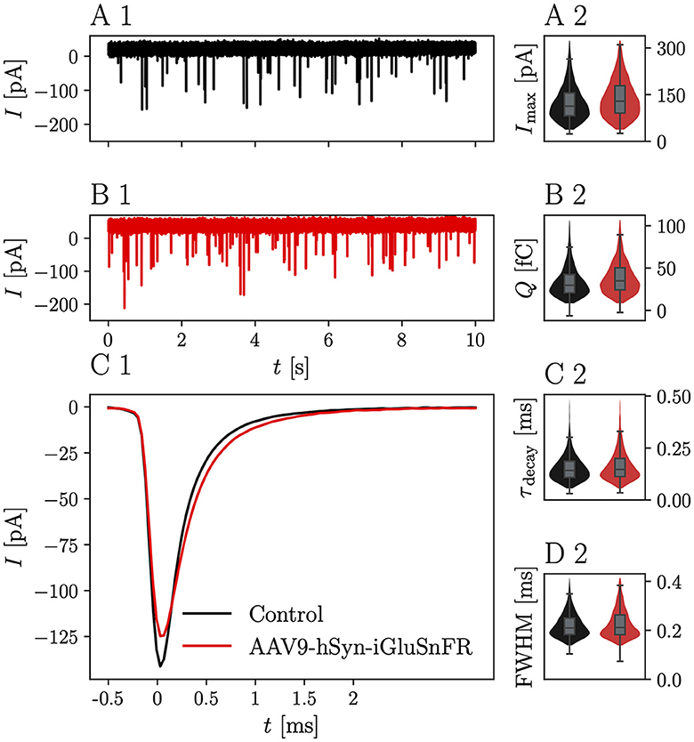
3.2 iGluSnFR expression prolongs the time course of mEPSCs

To address putative effects of iGluSnFR expression on synaptic transmission, we first analyzed spontaneous synaptic events at the endbulb of Held. In the endbulb of Held synapse, spontaneous excitatory postsynaptic currents (sEPSCs) in acute brainstem slices are not affected by tetrodotoxin (Oleskevich and Walmsley, 2002). We equate them to AMPAR-mediated miniature excitatory postsynaptic currents (mEPSCs) and tested whether they are affected by potential perturbations caused by the expression of iGluSnFR in the presynaptic SGN.

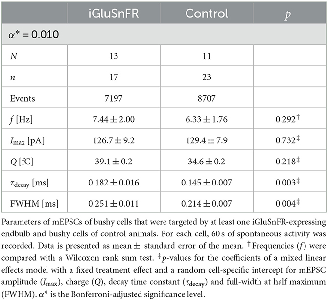
Representative mEPSC recordings from BCs, which were targeted by at least one iGluSnFR-expressing endbulb and control BCs are displayed in Figure 2A1. iGluSnFR expression was confirmed by a subsequent fluorescent response to monopolar stimulation, while control mEPSC recordings were made from uninjected littermates of the AAV-injected mice. Figure 2B1 shows average mEPSC waves of N = 13 animals, n = 17 cells in the injected group and N = 11 control animals (n = 23 cells), Figure 2C1 shows averaged single mEPSCs for the iGluSnFR group and control group and the kinetic parameters of the mEPSCs are presented in Figures 2A2–D2 and Table 1. While the mEPSC frequency, amplitude, and charge did not differ significantly, mEPSCs of BCs which were targeted by iGluSnFR-expressing ANFs decayed slightly slower (τdecay = 0.182 ± 0.016 ms) than mEPSCs of control cells (τdecay = 0.145 ± 0.007 ms, p = 0.003) and were slightly wider (full width at half maximum (FWHM) = 0.251 ± 0.011 ms) than control cells (FWHM = 0.214 ± 0.007 ms, p = 0.004).

Figure 2. iGluSnFR expression in the presynaptic membrane prolongs the mEPSC decay time without changing the overall glutamate charge. (A1) Shows a representative 10 s trace of a control BC held at -70 mV. (B1) Shows a corresponding trace of a BC which was targeted by at least one iGluSnFR-expressing SGN. (C1) Shows overlayed the average peak-aligned mEPSC for N = 13 animals and n = 17 cells in the iGluSnFR condition and N = 11 animals, n = 23 cells in the control condition. (A2–D2) Show violin plots with overlayed boxplots of the distribution of parameters of mEPSCs over all cells. The parameters are mEPSC amplitude (Imax), charge (Q), time constant of a single exponential fitted through the decay τdecay and full-width at half maximum (FWHM). For illustration purposes, violin plots were constrained to values within the 0.1–0.99 interquantile range. Boxes indicate the median, the 0.25 and 0.75 quantiles with whiskers spanning 1.5 times in interquartile range (outliers not shown).

Table 1. Measured and derived parameters of mEPSCs.

Assuming AMPARs are not saturated by a single quantum of glutamate (Ishikawa et al., 2002; Yamashita et al., 2003), an extracellular glutamate buffer, prolonging the time course in the synaptic cleft, while leaving the total amount of glutamate released unaffected, would alter the time profile of the postsynaptic currents, but not the integrated charge. According to this hypothesis, we expect the peak current to be reduced under the influence of iGluSnFR. This, however, was not observed to a statistically significant degree.

A caveat of our analysis is that mEPSCs recorded in a given BC may originate from synapses that vary in iGluSnFR expression. During some experiments on slices of AAV-injected animals, BCs with large eEPSCs failed to show any iGluSnFR fluorescence increase (data not shown). Even though these recordings were not included in the analysis of evoked release, their presence highlights the possibility that of the multiple endbulbs projecting onto the same BC, some did not express iGluSnFR. Since we ensured single-fiber stimulation and excluded recordings without iGluSnFR fluorescence increase, iGluSnFR-negative endbulbs did not contribute to the eEPSCs we measured. Yet, spontaneous release from iGluSnFR-negative endbulbs is expected, hence only a fraction of the measured quantal events originated from iGluSnFR-expressing endbulbs. Consequently, the differences may be a lower bound of the effect of iGluSnFR expression on single synapses.

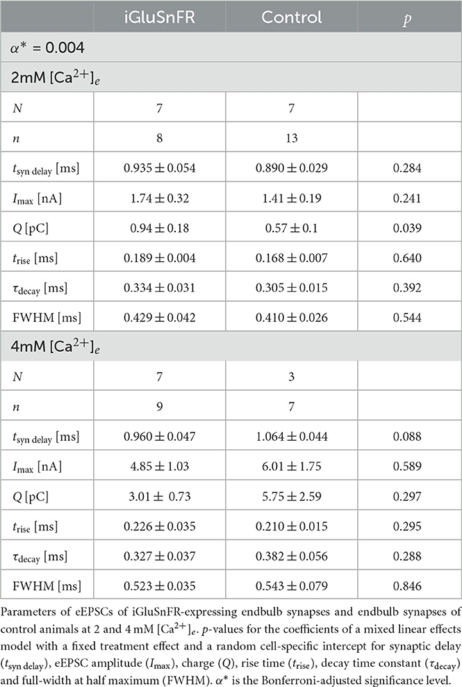
3.3 iGluSnFR expression does not alter evoked EPSCs

Given the effect of iGluSnFR expression on quantal currents, we further investigated possible effects on synaptic transmission by analyzing evoked release. In the endbulb of Held, monopolar stimulation is able to induce eEPSCs in the nA range, corresponding to the synchronized release of several tens to hundreds of SVs. Comparing the response of BCs postsynaptic to iGluSnFR-expressing and control endbulbs to a single electrical stimulus, we did not find significant differences in amplitude and kinetics (summarized in Table 2).

Table 2. Measured and derived parameters of eEPSCs.

At 2 mM [Ca2+]e we compared eEPSCS in BCs (n = 8) of AAV-injected mice (N = 7) to those of uninjected littermates (N = 7, n = 13). While the amplitude of eEPSCs tended to be larger in BCs of injected mice, the difference was not statistically significant (Imax, iGluSnFR = 1.74±0.32 nA, Imax, Control = 1.41± 0.19 nA, p = 0.241 at α* = 0.004).

We then measured eEPSCs at 4 mM [Ca2+]e (AAV-injected group: N = 7, n = 9, control group: N = 3, n = 7). The EPSC size in the AAV-injected group increased from 1.74 ± 0.32 nA at 2 mM [Ca2+]e to 4.85 ± 1.03 nA at 4 mM [Ca2+]e (p < 0.001). Likewise, in the control group, eEPSC sizes increased from 1.41 ± 0.19 nA to 6.01 ± 1.75 nA (p < 0.001). Comparison at 4 mM [Ca2+]e, did not reveal statistically significant differences (Imax, iGluSnFR = 4.85 ± 1.03 nA, Imax, Control = 6.01 ± 1.75 nA, p = 0.589). Neither at 2 mM [Ca2+]e, nor at 4 mM [Ca2+]e, we saw a statistically significant change in charge, FWHM, rise time, decay time constant and synaptic delay (see Table 2).

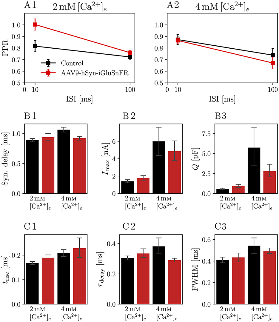
We then analyzed the eEPSCs to repetitive stimulation in the same iGluSnFR-expressing and control endbulbs. First, we considered the paired-pulse ratio (PPR), i.e. the ratio of two consecutive EPSCs with a defined inter-stimulus interval (ISI), presented in Figure 3. Comparing the PPRs with ISIs of 10 ms and 100 ms (see Figure 3 and Table 3) in 2 mM [Ca2+]e conditions revealed a statistically significant increase in the PPR10ms (PPR10ms, Control = 0.82 ± 0.05 and PPR10ms, iGluSnFR = 1.00 ± 0.05 p = 0.004) in endbulb synapses of injected mice, which was absent at a longer ISI.

Figure 3. Paired pulse ratio (PPR) of iGluSnFR-expressing endbulb synapses is increased for 10 ms interstimulus interval (ISI) at 2mM[Ca2+]e, but remains unchanged at higher calcium concentrations or longer ISIs. Plots show the PPR for ISI of 10 ms (PPR10ms) and 100 ms (PPR100ms) of N = 7 animals, n = 8 cells in the iGluSnFR group and N = 7 animals, n = 13 cells in the control group under 2mM[Ca2+]e conditions [in (A1)], and N = 7 animals, n = 9 cells in the iGluSnFR group and N = 3 animals, n = 7 cells in the control group at 4mM[Ca2+]e [in (A2)]. (B, C) Show bar plots with of kinetic parameters of EPSCs, namely synaptic delay (B1), eEPSC amplitude [Imax, (B2)], charge [Q, (B3)], rise time [trise, (C1)], time constant of a single exponential fit through the decay phase of the eEPSC [τdecay, (C2)] and full-width at half maximum (FWHM, (C3)]. Bars represent means ± standard error of the mean of the median values per cell.

Table 3. Comparisons of PPRs.

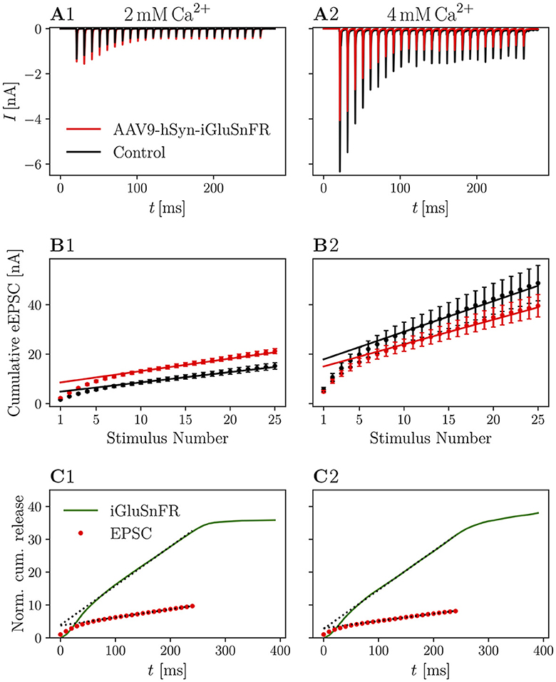
In order to assess potential differences in presynaptic activity, we further analyzed data collected from stimulus trains. If the expression of a transmembrane protein in the presynaptic membrane had an effect on the release of SVs, standard estimates of vesicle pool parameters might reflect these perturbations. Furthermore, if iGluSnFR was saturated with glutamate within the first few stimuli and stayed saturated for the remaining train, the current elicited by one SV in the beginning of a train, might be different from the current elicited by one SV in the end of the train, leading to differences in standard cumulative plots used to analyze high-frequency train data [Schneggenburger/Meyer/Neher (SMN) analysis (Schneggenburger et al., 1999)].

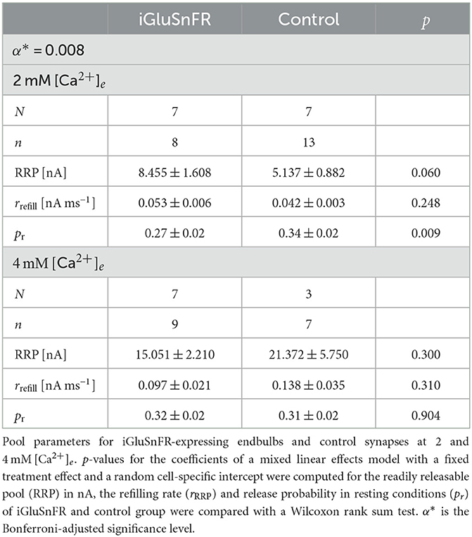
In Figure 4, recordings of 25 stimuli at 100 Hz are shown. The averaged raw traces (Figures 4A1, A2) and current amplitudes (Figures 4B1, B2) show the characteristic increase of release at elevated [Ca2+]e concentrations and the increase in PPR10ms at 2 mM [Ca2+]e. There was no significant change in pool parameters or release probability derived from the cumulative plots, summarized in Table 4.

Figure 4. Cumulative release is not significantly altered in iGluSnFR-expressing synapses and cumulative release analysis of iGluSnFR data is comparable to standard electrophysiological approaches. (A) Shows the absolute amplitude of eEPSCs elicited by 25 stimuli at 100 Hz, while in (B) the cumulative EPSC amplitude is plotted over the stimulus number in order to obtain estimates for RRP size, release probability and replenishing rate (see Schneggenburger et al., 1999; Neher, 2015). In (C), cumulative release derived from iGluSnFR recordings and eEPSC recordings from injected animals are plotted over time. The dashed line shows the fit of the steady-state response, continued to the ordinate. Error bars omitted for clarity. In (A1–C1) the data recorded from N = 7 animals, n = 8 cells in the iGluSnFR group and N = 7 animals, n = 13 cells in the control group [in (A, B)] under 2 mM [Ca2+]e conditions is shown. In (A2–C2), data recorded from N = 7 animals, n = 9 cells in the iGluSnFR group and N = 3 animals, n = 7 cells in the control group [in (A, B)] at 4 mM [Ca2+]e is shown.

Table 4. Pool parameters derived from cumulative eEPSCs.

3.4 Glutamate imaging yields quantitative measures of synaptic depression

To assess the feasibility of measuring evoked glutamate release with a GEGI and the validity of its use for estimating parameters of synaptic release, we systematically correlated iGluSnFR measurements with electrophysiological read-outs of glutamate release at 2 mM [Ca2+]e (N = 7 animals, n = 8 cells) and at 4 mM [Ca2+]e (N = 7, n = 9).

Since the signal-to-noise ratio (SNR) of iGluSnFR recordings was not sufficient to resolve the release of single SV in the preparation in our hands, we aimed for a robust protocol correlating electrophysiological and iGluSnFR recordings. This was achieved by measuring synaptic responses to single fiber stimulations both by fluorescence imaging at a frame rate of 100 Hz (Figures 5A, C) and voltage-clamp recordings of eEPSCs (Figures 5B, D). The peak ΔF/F