Measurement error can produce substantial bias and flawed inferences,1–8 but is often ignored.9 The importance of addressing measurement error increases as the use of routinely collected healthcare data for research becomes increasingly common.10 The primary purpose of these data is individual patient care, so some variables may be subject to greater measurement error than would be found in prospective research studies.11

Approaches to address measurement error commonly rely on validation data to estimate measurement error parameters (e.g., sensitivity and specificity).3,4,12 Validation data may be internal, that is, the validation sample is a sample of individuals from the main study sample and the validation sample does not include any individuals not included in the study sample, or validation data may be external, that is, the validation sample includes individuals not included in the main sample. Prospective collection of validation data can be costly and time-consuming. Thus, the use of existing data as validation data is an attractive alternative. However, existing data are almost always external to the main study sample, so we need to consider how to “transport” measurement error parameters from the validation sample to the study sample (Sec. 2.2.4 in 3).12,13

Here, we introduce estimators that transport measurement error parameters from external data to account for misclassification of outcomes in the study sample. We specifically focus on the setting where there is no overlap between the external validation sample and the study sample. We apply the estimators in a motivating example to account for misclassification in preterm birth in a sample of pregnant people in Lusaka, Zambia, captured in an electronic health record, leveraging more accurate preterm birth measurement data from external research studies.

METHODS Motivating Example

We aimed to estimate the overall risk of preterm birth (i.e., the natural course14) and the causal effect of maternal HIV infection on the risk of preterm birth among people seeking prenatal care in Lusaka, Zambia. We use data from the Zambia Electronic Perinatal Record System (ZEPRS), an electronic health record used by 25 clinics and one referral hospital in Lusaka with deliveries between 1 January 2008 and 26 June 2013.15,16 These data are our study sample.

In ZEPRS, the outcome of preterm birth was defined by gestational age at birth <37 weeks, as measured by patient-reported last menstrual period (LMP). However, LMP-derived gestational age is subject to nontrivial measurement error17–25 that typically results in an overestimate of preterm birth risk.26–30 In contrast, gestational age derived from an early ultrasound is a more accurate measure,23,30–35 but this technology is not routinely available in these prenatal care clinics. Therefore, outcome misclassification is a concern in our study sample.

More recently (2015–2020), two research studies prospectively enrolled a nonrandom sample of pregnant people at clinics where ZEPRS had been deployed.36,37 These studies assessed preterm birth by both LMP and early ultrasound and are used herein as a validation sample. The validation sample is considered external because it includes individuals who were not in the study sample. In fact, there is no overlap in the samples because the time periods of the studies differ.

Accounting for Outcome Misclassification

Let Y and A be binary indicators for the true outcome (e.g., preterm birth) and exposure (e.g., HIV infection), respectively. We aimed to estimate the marginal risk of the outcome under the natural course and two counterfactual marginal risks, one for the scenario where everyone was exposed and one for the scenario where everyone was unexposed, in the study sample (which we assume is a random sample of the target population). The natural course is denoted P(Y=1|R=1) and the counterfactual risks are denoted P(Y(a)=1|R=1), where Y(a) is the potential outcome (i.e., the outcome that would be observed) when A=a and R is an indicator of whether the person was in the study sample, R=1, or in the validation sample, R=0. Let Z be confounders (i.e., common causes of A and Y). Under conditional exchangeability for confounding with positivity and causal consistency,38–41 we can identify the counterfactual risks using the g-formula,38

P(Y(a)=1|R=1)=∑z⁡P(Y=1|A=a,Z=z,R=1)P(Z=z|R=1).

For simplicity, our notation assumes categorical Z.

However, only Y∗, a potentially misclassified version of Y, was measured in our study sample. To account for misclassification, we can replace P(Y=1|A=a,Z=z,R=1) in equation [1] with42,43

P(Y∗=1|A=a,Z=z,R=1)−(1−SpA,Z,R=1)SeA,Z,R=1−(1−SpA,Z,R=1),

where SeA,Z,R=1=P(Y∗=1|Y=1,A=a,Z=z,R=1) and SpA,Z,R=1=P(Y∗=0|Y=0,A=a,Z=z,R=1) are the misclassification parameters sensitivity and specificity, respectively, stratified by A and Z in the study sample (proof in eAppendix; https://links.lww.com/EDE/C94). However, misclassification parameters in the study sample (i.e., when R=1) are not identified from the observed data since Y is missing. In contrast, misclassification parameters are identified in the validation sample (i.e., when R=0). To replace the misclassification parameters from the study sample in equation [2] with the misclassification parameters from the validation sample, we must consider whether the parameters are transportable. By transportable, we mean that the misclassification parameters in the validation sample equal those in the study sample, either unconditionally (i.e., marginally) or conditional on covariates.

When R is independent of Y∗ conditional on Y, A and Z (R∐Y∗|Y,A,Z), the A and Z conditional misclassification parameters are transportable.

P(Y∗=y∗|Y=y,A=a,Z=z,R=1)=P(Y∗=y∗|Y=y,A=a,Z=z,R=0).

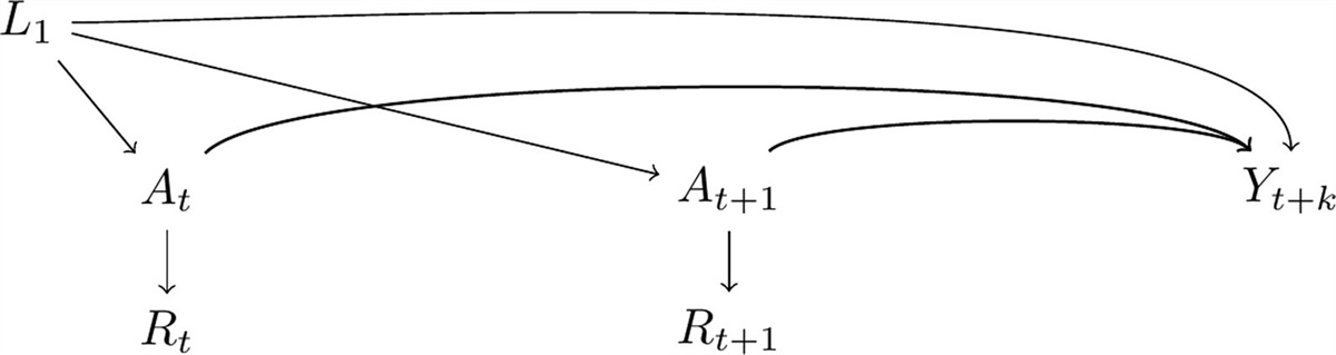
R∐Y∗|Y,A,Z is a conditional exchangeability assumption for transportability. Figure 1A,B are causal diagrams where this assumption holds. We also require a positivity assumption—that is, the validation sample includes individuals across the observed distribution of A and Z in the study sample (i.e., P(R=0|Z=z,A=a)>0 for all a,z where f(a,z|R=1)>0, where f is the density).44

FIGURE 1.: Causal diagrams for simulation scenarios.

ϵy

is the measurement error. Arrows from

R

into other nodes signify that the distributions of

A

,

Z

,

Y

, and

W

differ between the external validation data and study sample indicated by

R

.

In the special case when misclassification is nondifferential with respect to A and Z, (A,Z∐Y∗|Y,R; Figure 1A), then sensitivity and specificity are constant across Z and A and we can replace conditional misclassification parameters with marginal parameters in equation [2] (i.e., P(Y∗=y|Y=y,A=a,Z=z,R=1)=P(Y∗=y|Y=y,R=1)) and the parameters are unconditionally transportable in equation [3] (i.e., P(Y∗=y|Y=y,R=1)=P(Y∗=y|Y=y,R=0)). This assumption does not hold in Figure 1B, where misclassification is differential with respect to A and Z.

Relaxing the Transportability Assumption

In Figure 1C, misclassification is differential with respect to nonconfounding covariates W (arrow from W to ϵy) and the distribution of W varies across the samples (arrow from S to ϵy). In this setting, our conditional exchangeability assumption for transportability introduced above does not hold (R∐Y∗|Y,A,Z) and thus the equality in equation [3] does not hold. Intuitively, even conditional on A and Z, the different distribution of W across the samples results in different misclassification parameters across the samples. In our motivating example, measurement error in LMP-measured gestational age may be differential by birth history30 (e.g., nulliparity) and the distribution of birth history may vary between the validation and study samples (e.g., the proportion nulliparous may differ). In the presence of these W covariates, the misclassification parameters are transportable if we additionally condition on W,

P(Y∗=1|Y=1,A,Z,W,R=1)=P(Y∗=1|Y=1,A,Z,W,R=0).

This equality holds under a relaxed conditional exchangeability assumption for transportability, R∐Y∗|Y,A,Z,W, with positivity across the observed distribution of A, Z, and W in the study sample. For Figure 1C, we focus on two identification approaches.

In the first approach, we condition on and standardize by both Z and W (hereafter called conditioning on W) in equation [1]: P(Y(a)=1|R=1)=∑z,w⁡P(Y=1|A=a,Z=z,W=w,R=1)P(Z=z,W=w|R=1). Consequently, equation [2] is also conditional on W and our sensitivity and specificity can be transported (proof in eAppendix; https://links.lww.com/EDE/C94). By conditioning on W, our conditional exchangeability assumption for confounding is now Y(a)∐A|Z,W (as opposed to the original Y(a)∐A|Z).

In the second approach, we condition on W in the outcome model only and take an expectation of the outcome model over W,

P(Y(a)=1|R=1)=∑z⁡E[P(Y=1|A=a,Z=z,W=w,R=1)|A=a,Z=z,R=1]P(Z=z|R=1),

(hereafter called the iterated approach). Similarly to conditioning on W, equation [2] is now conditional on W and our sensitivity and specificity can be transported (proof in eAppendix https://links.lww.com/EDE/C94). Differently than conditioning on W, the iterated approach includes iterated expectations and thus relies on the original conditional exchangeability assumption for confounding, Y(a)∐A|Z.

A third identification approach that involves standardization of the validation sample to the W-distribution of the study sample (and a corresponding weighted estimator) is provided in the eAppendix; https://links.lww.com/EDE/C94. This approach requires a strong assumption of independence of W and Y, which is unlikely to be met in practice; therefore, we do not consider this approach further.

The identification assumptions for (1) conditioning on W and (2) the iterated approach, hold in Figure 1C, but only the assumptions for the iterated approach hold in Figure 1D where W is a collider on a closed backdoor path from A to Y. In the conditioning on W approach, conditional exchangeability for confounding does not hold because conditioning on W opens the backdoor path from A to Y inducing M-bias.45 Therefore, risk differences are not identified, though we can still identify the natural course risk as conditional exchangeability for confounding is not required. The iterated approach does not induce M-bias because the conditional exchangeability for confounding assumption is not conditional on W.

Estimation

When Z is low-dimensional and there are enough data, we can estimate all quantities nonparametrically. Otherwise, we use parametric models, at the cost of requiring that the models are correctly specified. See eAppendix; https://links.lww.com/EDE/C94 for details. Estimation with parametric models follows these steps:

Estimate the misclassification model in the validation sample using a logistic model where Y∗ is the outcome and the model includes Y, A, and Z (and interactions). Use the estimated misclassification model to obtain estimates of sensitivity and specificity for each individual in the study sample by setting Y=1 and Y=0. Estimate the outcome model in the study sample. One approach follows equation [2] and we can use a logistic model to estimate the misclassified outcome model in the study sample, P^(Y∗=1|A=a,Z=z,R=1), however, this implementation requires estimating sensitivity and specificity values under each value of a and under the natural course (in step 2). An alternative approach avoids estimation of these “potential” sensitivities and specificities by directly estimating the outcome model in the study sample (as in Equation [1]), P^(Y=1|A=a,Z=z,R=1), by maximizing a likelihood of the observed data that leverages the estimated sensitivity and specificity (eAppendix; https://links.lww.com/EDE/C94).12,46,47 We use this latter approach, which also extends to multinomial outcomes (eAppendix; https://links.lww.com/EDE/C94). Generate predictions from the estimated outcome model for the study sample under a specified distribution of A (e.g., observed A values for the natural course, A=1 for all exposed). Take the mean of the predictions to estimate the corresponding risk.48

When misclassification is differential with respect to W and the distribution of W differs across the samples, we can either (1) condition on W or (2) use the iterated approach. For both approaches, W is included in the misclassification model estimated in step 1 and in the outcome model estimated in step 3. For the conditioning on W approach, all the other steps are the same. In contrast, the iterated approach includes additional steps immediately after step 4:

4.1 Estimate another logistic model (hence the name iterated) in the study sample where the prediction from step 4 (from the outcome model conditional on W) is the outcome. 4.2 Generate predictions from the model estimated in step 4.1 for the study sample under a specified distribution of A (the same distribution as used in step 4).

After these two additional steps (4.1 and 4.2), implement step 5 above (take the mean of the predictions to estimate the risk).

Estimation of the variance ought to account for uncertainty in the misclassification parameters estimated in the validation sample. One option is nonparametric bootstrap in which both samples are independently resampled.49 Instead, we use M-estimation and the empirical sandwich variance estimator (eAppendix; https://links.lww.com/EDE/C94),50,51 which is more computationally efficient than bootstrap.

Simulations

We conducted illustrative simulations. We generated data loosely based on our motivating example for 5000 cohorts under each of the four scenarios depicted in Figure 1 (eAppendix; https://links.lww.com/EDE/C94, code available at https://github.com/rachael-k-ross/MeasurementError-ExternalValidation). In the original data generation for Figure 1D, the U nodes had a modest impact on the other nodes (odds ratio 1.2). It has been shown that meaningful M-bias requires strong relationships along the “M” path.45 Thus, to emphasize the potential M-bias from conditioning on a collider (in the Conditioning on W approach), we also present results under an altered data generation in which the U nodes have a strong impact (odds ratio 4.0) (eAppendix; https://links.lww.com/EDE/C94). For each scenario, we conducted six analyses using the estimators described above to estimate the natural course outcome risk and the marginal causal risk difference: (0) using the true outcome Y (although impossible in practice, this provides a benchmark); (1) using the misclassified outcome Y∗; (2) accounting for nondifferential misclassification in Y∗; (3) accounting for differential misclassification with respect to A and Z; and accounting for differential misclassification with respect to A, Z, and W by (4) conditioning on W or (5) the iterated approach. To describe performance, we estimated bias, empirical standard error (ESE), average estimated standard error, and 95% confidence interval (CI) coverage.