To investigate aircraft noise exposure trends by airport and populations exposed, we utilized noise exposure contours for U.S. airports, identified airport characteristics, and estimated exposed populations by race and ethnicity.

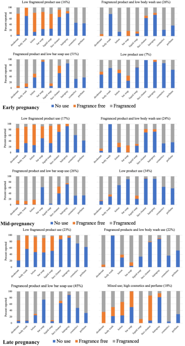
We obtained noise exposure contours for 90 U.S. airports (Fig. 1) from the U.S. Department of Transportation (DOT) Volpe National Transportation Systems Center (Volpe). The airports included in this study constitute 18% of the Part 139 U.S. Federal Aviation Administration (FAA) certified airports, but represent 88% of total enplanements in 2015 [26]. Noise contours were modeled for years 1995, 2000, 2005, 2010, and 2015. Detailed information on the generation of aircraft noise contours is provided elsewhere [24, 27]. Briefly, noise contours were created using FAA’s Aviation Environmental Design Tool (AEDT), which was developed using internationally accepted practices to estimate the environmental impact of aviation. Estimations were formulated with data (e.g., airport runway locations and utilization) from the Enhanced Traffic Management System (ETMS) for 2000–2015 and Official Aviation Guide (OAG) for 1995 and standard aircraft profile data in the Aircraft Noise and Performance (ANP) database.

Sample of U.S. airports (n = 90) included in the study.

We used two noise metrics in this study: DNL and Lnight. DNL reflects noise exposure for an average 24-h period of the year that artificially penalizes nighttime hours by adding 10 dB(A) to measurements from 22:00–07:00 when noise sensitivity may be higher due to lower ambient noise. Lnight reflects noise exposure summarized over nighttime hours. DNL and Lnight were modeled in one dB(A) increments ranging from 45–75 dB(A).

We focused on three noise thresholds: (1) DNL 65, (2) DNL 45, and (3) Lnight 45 dB(A) levels, the first of which relates to the U.S. regulatory threshold for significant noise exposure, and the latter two of which correspond to the World Health Organization recommended guidelines for aircraft noise exposure in the European region [5]. Our nighttime threshold is limited to the lowest available modeled data at 45 dB(A).

To exclude non-livable areas from the assessments, we overlaid the contours with national area hydrography (i.e., water bodies) and greenspace geodatabases. National area hydrography geodatabases (ponds, lakes, oceans, swamps, glaciers, rivers, streams, and/or canals) were available from the U.S. Census Topologically Integrated Geographic Encoding and Referencing (TIGER) database. Hydrography databases for 2013 [28] were overlaid with 1995–2010 noise contours, and for 2016 [29] with 2015 contours. A 2010 national greenspace layer (parks, gardens, and forests) was available from Esri [30] and overlaid with all contour years.

We identified various airport characteristics by the four U.S. Census regions (Midwest, Northeast, South and West) and FAA hub type designation from 2001 (passenger/cargo airline hub type, and cargo hub). FAA categorizes primary commercial airports (more than 10,000 passenger boardings each year) into hubs according to 49 U.S. Code § 47102, where large hubs receive greater than or equal to 1% of the annual U.S. commercial enplanements, medium hubs 0.25–1%, small hubs 0.05–0.25%, and nonhubs less than 0.05% but more than 10,000 passenger boardings per year [31]. Passenger/cargo airline hub type was categorized according to mainline passenger and cargo airline designations of airports. Concentrated LTO operations use hub-and-spoke, where airlines centralize regional operations to major central hubs, or point-to-point models, which are direct A–B operations that do not require passing through a central hub [32]. Airports were designated as primary if serving as a main central hub for a hub-and-spoke airline, secondary if serving as a support hub for a hub-and-spoke airline, focus city if designated as a focal airport for a point-to-point airline, or nonhub/focus city if not serving as a hub or focus city. We categorized airports as a cargo hub if ranked by the FAA as among the top 25 for all-cargo landed weights. Airport passenger enplanement and cargo data were available from the Bureau of Transportation Statistics for 1995 and from the FAA Air Carrier Activity Information System (ACAIS) database for 2000–2015 [33, 34]. LTO operations data were available from the Air Traffic Activity System (ATADS) database for 1995–2015 [35].

We first estimated mean changes in contour areas over time using response profile analyses across all 90 airports. The analysis of response profiles allows for characterizations of patterns of change in the mean contour area over time. This method is appropriate for longitudinal studies with a balanced design, when timing of repeated measures are uniform across subjects, and for data that violate assumptions of independence and homogeneity of variance [36]. Contour area data were complete for all 90 airports across each study time-point and were assumed to correlate across years by airport. Covariance structures were selected by examining fit statistics tables and likelihood ratio tests for nested models.

Rather than solely relying on fixed, a priori factors, identifying distinct groups of airports with shared characteristics could provide an informed approach for epidemiological studies to utilize different airport characteristics in exploring associations between aircraft noise exposure and health. We assessed variation between airports by statistically arranging airports by similarity using group-based trajectory modeling (GBTM). GBTM is a specialized application of finite mixture models that identifies distinct groups sharing underlying characteristics and trajectories [37]. We applied the SAS package Proc Traj with a beta regression, which is appropriate for non-normal distributions [38, 39]. The beta distribution dictates normalizing noise contour areas to fit within a zero to one range using the minimum and maximum area values within respective years [40]. Model parameters were estimated using maximum likelihood. To determine the optimal number of groups, we started with a one-group model and sequentially fitted an increasing number of groups in a stepwise manner. The best fitting model was selected using the following criteria: logged Bayes factor (2Δ BIC), Jeffreys’ scale of evidence for Bayes factors, non-overlapping confidence intervals, a posterior-probability of group membership greater than 0.7, and approaching a sufficient sample size of ideally ≥5% in each group [41, 42]. We simultaneously determined the shape of each trajectory over time (i.e., order of a polynomial relationship) using BIC values. We tested for nonrandom associations between characteristics and trajectory groups using Fisher’s exact test due to small cell sizes.

We evaluated changes in exposed populations overall, by Hispanic/Latino ethnicity, and race as defined by the U.S. Census. Using the U.S. Census designation, Hispanic/Latino ethnicity was categorized as those who identify as Hispanic or Latino versus non-Hispanic/non-Latino. Race was categorized as those who identified as White alone, Black or African American alone, Asian alone, American Indian/Alaska Native, Native Hawaiian/Other Pacific Islander alone, some other race alone, or two or more races. Population data were obtained at the Census tract level for 2000, 2005, 2010, and 2015 from GeoLytics Inc. After 2001, inter-decennial Census categorizations for race excluded “some other race” and reapportioned “some other race” and part of “two or more races” into remaining races. For consistency of race categories over time we used race counts from the decennial Census for 2000 and 2010 and the 5-year American Community Survey (ACS) estimates for 2005 and 2015. All Census and ACS data were aligned at the 2010 census tract boundaries for comparative analysis from 2000–2015. Data for year 2000 and 2015 were available from GeoLytics preweighted to 2010 boundaries, while 2005 data were interpolated to 2010 boundaries using geographic crosswalks available from IPUMS National Historical Geographic Information System [43]. We estimated number of people residing in areas of noise exposure using simple area weighting, which sums the proportions of masked noise contour areas that overlap with tracts multiplied by the population estimates within overlapping tracts.

Exposed population estimates were evaluated in the following ways: (1) normalized by the tracts’ respective sub-population; (2) by absolute counts; and (3) normalized by the tracts’ total population. Tracts were selected (n = 13,416) if they intersected the largest noise exposure contour during our study period (DNL 45, dB[A] for 2000); we defined these tracts as “living close to airports”. We normalized by tract sub-populations to assess whether there was a disproportionate burden of exposure on racial/ethnic groups (e.g., exposed Hispanic/Latino population normalized by the total Hispanic/Latino population living within the tracts around the airport), and normalized by the tract total population in order to account for overall changes in population growth/decline.

In order to determine if the sociodemographic characteristics of the population exposed to aircraft noise differed by airport characteristics over time, we also examined changes in counts and normalized proportions of exposed populations when stratified by trajectory groups. We hypothesized that this analysis would provide insight into the association between the shared underlying properties determining aircraft noise exposure trajectories and demographic characteristics, such as ethnicity and race, of exposed populations.

Spatial analyses were completed using a common projected coordinate system within a geographic information system (GIS; Esri ArcGIS® Pro V2.2.3; Redlands, California). Geographic areas were estimated in units of square kilometers (km2) after masking. Statistical analyses were performed using Statistical Analysis System (SAS) v9.4 (Cary, North Carolina).