We retrospectively studied patients > 18-years-old who were surgically treated due to acute ankle fractures (OTA/AO 44) between 2015 and 2023 at a tertiary referral hospital. Analyses were done on the basis of their medical and imaging records. Our study was approved by the institutional review board (IRB) of our institution.

Inclusion criteria were the presence of malleolar fractures in adult patients who were surgically treated with open reduction and internal fixation (ORIF). All participants had both standard anterior–posterior and lateral views of ankle radiographs. Exclusion criteria included no available preoperative scan of computed tomography (CT), incomplete set of radiographs, age < 18-years-old, open fractures, prior surgeries with implants at the ankle, pathologic ankle fractures, tibial pilon fracture (OTA/AO 43), and ankle injuries without malleolar fractures.

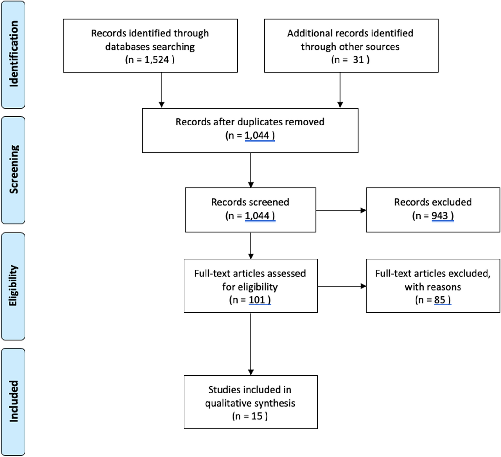
From the 565 initially eligible cases, we finally included a total of 156 cases for further analysis. On the basis of the exclusion criteria, 413 patients were dropped as most of these excluded cases had no preoperative CT image. Among them, 14 out of 229 cases (6.1%) were unimalleolar fractures, and 17.3% were bimalleolar fractures with preoperative CT, while 72.6% of trimalleolar fracture cases had complete preoperative images. As a result, a total of 156 patients were included for this study. Of 156 ankle fractures, 109 (69.9%) were trimalleolar fractures, 33 (21.1%) were bimalleolar fractures, and 14 (9.0%) were unimalleolar fractures, according to Pott’s classification. The flow chart of case selection is presented in Fig. 1. For further analysis, we extracted from medical records, information on patients’ baseline characteristics, such as age, sex, body weight, and height, side of ankle injury, trauma mechanism, prior medical history including diabetes mellitus (DM) and end-stage renal disease (ESRD), American Society of Anesthesiologists (ASA) classification, syndesmosis separation, the fracture patterns further classified on the basis of Denis/Weber, Lauge-Hansen classifications and posterior pilon variants, and complications.

Flow chart of enrolled cases

Traumas are divided into two categories based on injury mechanisms: low energy, and high energy traumas, according to the high energy trauma criteria proposed by Guzmán-Juárez et al. [15]. High energy trauma includes: (1) accident in a motor vehicle with a speed > 60 km/h (or 37 mph); (2) motor vehicle accident in which the vehicle rolled over; (2) person ejected from vehicle; (3) pedestrian hit by a vehicle at a speed > 10 km/h (or 6.2 mph); (3) cyclist hit at a speed > 20 km/h (or 12.4 mph); (4) hit by a motorized vehicle at a speed > 30 km/h; and (5) drop from a height > 5 m (or 16.4 ft). Other injury mechanisms are considered related to low energy traumas.

We used standard radiologic criteria in this study. All radiographic parameters were measured using the image-builtin software, the picture archiving and communications system (PACS) provided by Ultraquery (Taiwan Electronic Data Processing, Sindian City, Taiwan). Ankle fractures were diagnosed on the basis of simple radiographs (both anteroposterior and lateral views) and CT scans with the three-dimensional (3D) reconstruction feature (3D-CT). Fractures were determined according to the classifications of Pott’s, Lauge-Hansen, and Danis-Weber.

According to Hunt’s report of 2013, the normal cut-off value of radiographic tibiofibular clear space is 5 mm. Hence, syndesmosis separation is diagnosed if the tibiofibular clear space is ≥ 6 mm [12].

We used Pott’s classification system based on the number of fractured malleoli in an ankle fracture, with a maximum of three involved malleoli (medial malleolus, lateral malleolus, and the posterior malleolus) [16]. Danis-Weber and Lauge-Hansen classifications were also utilized in this study to classify the ankle fractures patterns [17]. Two experienced orthopedic surgeons independently reviewed all imaging studies, including fracture classifications and identification of AITFL avulsion. Discrepancies were resolved based on the findings of CT scan by discussion.

Posterior malleolus fractures with posterior pilon fracture were defined with respect to tibial incisura involvement according to the system of Barton´ıcek et al. and Switaj et al. [18, 19]. Cases were identified as the posterior pilon fracture if the posterior malleolar fracture had involved the whole tibial metaphysis, and exiting the medial malleolus through the posterior colliculus. Radiological signs of posterior pilon fractures on both anteroposterior and lateral radiographs containing posterior subluxation and double contour sign at the medial malleolus, i.e., involving the whole tibialis posterior metaphysis would have led to a double joint line sign [19].

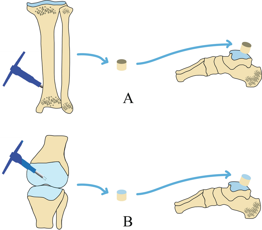
Following classification of the ankle fracture, the presence of AITFL avulsion fractures was determined based on the preoperative CT-scan, and mainly according to a Modified Wagstaffe classification [6]. (Fig. 2a) Type I referred to an isolated AITFL avulsion fracture of the fibula without lateral malleolar fracture; type II referred to AITFL avulsion fracture of the fibula with lateral malleolar fracture; AITFL avulsion fracture of the tibia was classified as type III which represented an additional type outside the original Wagstaffe classification; finally, type IV represented AITFL avulsion fracture involving both tibia and fibula. Moreover, we also classified the AITFL avulsion fractures using the original Wagstaffe classification [13]. (Fig. 2b).

The classification of AITFL avulsion fractures: a modified Wagstaffe classification, b original Wagstaffe classification [14, 21]

Wagstaffe avulsion fracture was defined as the avulsion fracture of the Wagstaffe tubercle on the anterior distal fibula, and Chaput avulsion fracture as the avulsion fracture of the Chaput tubercle on the anterior distal tibia, with both tubercles representing the insertion of the anterior inferior tibiofibular ligament [7] (Fig. 3). An example of a 70-year-old female with AITFL avulsion fracture in ankle fracture is illustrated in Fig. 4.

The Wagstaffe and Chaput avulsion fractures

Ankle fracture with AITFL avulsion fracture. A 70-year-old female with left trimalleolar fracture, but Wagstaffe avulsion fracture is only visible on the lateral view of ankle standard radiograph (a and b, yellow arrow). On the other hand, both Wagstaffe and Chaput avulsion fracture can be easily identified on different CT views c–f, including coronal, axial, sagittal and an ankle three-dimensional computed tomography image. Yellow arrows indicate Wagstaffe avulsion fracture; white arrows indicate Chaput avulsion fracture

All analyses were performed on the IBM® Statistical Package for the Social Sciences (SPSS®), version 22. Continuous data were presented as means and standard deviations. Their normality of distribution was assessed with the Kolmogorov–Smirnov test. The Mann–Whitney U test was performed to examine intergroup differences in age, height, weight, and body mass index (BMI). Descriptive data, such as patients’ sex, and side of ankle fracture, were presented as frequencies and percentages. The chi-square analysis and Fisher’s exact test were conducted to compare categorical data between the two groups. Statistical significance was set at p < 0.05. Differences in baseline characteristics between patients with and without AITFL avulsion fractures were analyzed using Mann–Whitney U test for continuous data. Chi-square analysis and Fisher’s exact test were used to compare categorical data between the two groups. Within the study population, the incidence of AITFL avulsion fractures was defined. To investigate the correlation between the type of ankle fracture and the type of AITFL avulsion fracture, 2 × 2 contingency tables were generated and significance was assessed using the Chi-square analysis and Fisher’s exact test. Logistic regression was performed for risk factor identifications for AITFL avulsion fractures. To determine the statistical power of our study, we used G*Power 3.1.9.7 (Heinrich Heine University, Düsseldorf, Germany) for analysis.