Study cohort

This study was performed according to an institutional review board (IRB) approved protocol. Forty-four atrial fibrillation (AF) patients (Table 1) were retrospectively recruited and underwent cardiac MRI, including LA 2D RTPC with through-plane velocity encoding. Inclusion criteria was a history of AF or AF patients who had previously underwent an ablation ( > = 3 months prior to the study). No patients received an ablation during the study. Five AF patients underwent a second cardiac MRI as part of a test and retest reproducibility (mean time between scans 13 ± 5 days), for a total number of 49 AF patient data sets available for LA flow analysis. No patients had prior left atrial appendage closures, clipping, or ligation. Patients were excluded if they had MRI contraindications, were pregnant, had severe claustrophobia, were non-English speakers, or were unwilling or unable to give informed consent. All patients gave informed consent in writing.

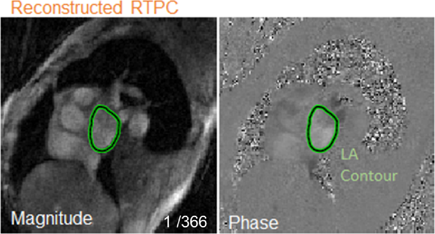
Table 1 Patient demographics across training and testing. Race was self-reported by the patientMR imaging

All subjects were scanned on a 1.5T MRI system (Siemens MAGNETOM Aera or Siemens MAGNETOM Avanto Erlangen, Germany). Cardiac MRI included anatomic and flow imaging of the LA. 2D RTPC imaging planes were placed at the mid LA oriented parallel to the mitral valve with through plane velocity encoding (Fig. 1). EKG R-waves detected by the scanner’s physiological measurement unit (PMU) were recorded in the 2D RTPC raw data header to delineate each heartbeat in subsequent analysis.

Fig. 1

LA RTPC plane is placed parallel to the mitral valve. 2D RTPC raw data is reconstructed into magnitude and phase cardiac data based on acquisition time (366 frames total for this patient). The left atrium is contoured to quantify blood flow velocities. LA- left atrium

The 2D RTPC data were acquired using a previously described highly undersampled pulse sequence [14]. Data were acquired during free breathing using a gradient-echo sequence employing radial k-space sampling with golden angles (111.2461°) with the following acquisition parameters: venc = 60–70 cm/s, acquisition matrix size 192 × 192, field of view (FOV) = 288 mm x 288 mm, flip angle = 8°, spatial resolution = 2.1 mm x 2.1 mm, slice thickness = 7–8 mm, TE = 2.88 ms, TR = 4.25 ms, acceleration factor R = 28.0, and total acquisition time varied from 5 to 20 s.

As described previously in Haji-Valizadeh et al., undersampled k-space data were reconstructed offline using the GRAPPA operator gridding Golden-angle Radial Sparse Parallel (GROG-GRASP) method [14, 22]. Temporal total variation was used as the sparsifying transform with normalized regularization weight 0.0078 (relative to the maximum signal of the time-averaged image) and 22 iterations. Each image was reconstructed with 5 radial k-space lines per time frame, with interleaved reference and velocity-encoded acquisitions for each k-space line, resulting in an effective temporal resolution of 42.5 ms (= TR x 2 × 5).

Semi-automated RTPC flow analysis

For LA flow quantification, a semi-manual processing pipeline was used to delineate the outline of the LA on 2D RTPC magnitude images for all time frames for each patient (Fig. 1). The LA was manually contoured on the first time frame to determine a seed region as input for a magnitude intensity-based region growing algorithm (Matlab, Mathworks). This seed region was then propagated to all time frames and region growing was subsequently applied. Next, each time frame was manually reviewed, and a human observer could modify the LA contour, typically removing excess contoured areas encroaching into the pulmonary vein, left ventricle, or aorta. Alternatively, the observer could add to the contoured area, typically near the LA wall. These LA contours served as ground truth labels for training and testing of the deep learning network for fully automated LA contouring. Furthermore, to assess inter-observer variability, the semi-automated analysis was repeated for twelve patients by a second observer, blinded to the results of the first reader.

Convolutional neural network design for 2D RTPC LA contour delineation

A 3D U-Net network [23] with DenseNet-based dense blocks [24], replacing the typical U-Net convolutional layers was utilized to segment the LA (Fig. 2). This network was adapted based on a previous network for 3D segmentation of the thoracic aorta [25]. Previously validated hyper parameters for the network (network depth, layer design, optimizer, and learning rate) were used, saving the computational effort of performing a nested cross validation scheme. Underscoring, the model weights, themselves, were zeroed and retrained. The hyper parameters used: a constant learning rate 0.001, ADAM optimizer, max pooling, a dropout rate of 0.1, skip connections from decoder to encoder sections, and channel size of 12. Dense blocks concatenated all prior feature maps for use as inputs to subsequent layers, which allowed for efficient feature reuse. Max-pooling was utilized for down sampling within the encoder structure and transposed convolution within the decoder structure. The final layer consisted of a 1 × 1 × 1 convolution and softmax function to generate a probability of each voxel (2D spatial + time) of the magnitude input image volume belonging to the LA or the background, and the LA contour was generated by selecting the class with the highest probability. A composite loss function composed of minimizing the equal sum of the softmax-cross entropy and complement of Dice score during training was utilized. During training and validation, an identical network with long short term memory (LSTM) blocks was trained and compared to the above network. Deep learning networks were developed in Python 3.6.8 (Python Software Foundation, Beaverton, OR) using Tensorflow 1.12.0 (Google, Mountain View, CA). Training time was 36 min. Training and testing of the deep learning network was performed on a NVIDIA GeForce GTX 1080 with an Intel i7-8700k processor.

Fig. 2

RTPC magnitude volume data (2D image data + time) is preprocessed and inputted into a dense U-net architecture convolutional neural network. The network features 2,4,6,8, 12 dense (outputs of each layer feed forward as inputs to subsequent) layers per layer with each layer consisting of batch, relu, convolution and drop out with constant feature map size of 12. Max-pooling was utilized for down sampling within the encoder structure and transposed convolution within the decoder structure. The final layer consisted of a 1 × 1 × 1 convolution and softmax function to generate a probability of each voxel (2D spatial + time) of the magnitude input image volume belonging to the left atrium or the background for each time frame

Reconstructed 2D RTPC data were automatically pre-processed prior to network input. Each patient’s 2D RTPC time series of magnitude images can be denoted as \(\:P(_\dots\:_\dots\:_)\) where \(\:_\) represents a magnitude image at timepoint t where \(\:t\in\:[1\dots\:T]\) and T is the total number of time frames for a patient P. Every magnitude image per patient was automatically center cropped to a fixed dimension of 96 × 96. Next, the data was automatically broken into multiple 50 time frame blocks with a 20 time frame overlap between neighboring blocks given by:

$$\:_\left(I\right)=\left\_\right)\right|\:i\in\:\left[30\left(j-1\right)+1\:.\:\:\:.\:\:\:.\:\:30\left(j-1\right)+51\right]\}$$

Where b is the jth block of 50 time frames. If the final block was less than 50 time frames, it was concatenated to the previous block. Frame overlap between blocks served to increase the number of training data set inputs and reduce input size compared to full patient data input, reducing GPU requirements. 50 time frames of data corresponded to a total time of 2125ms, covering multiple heartbeats. Images were normalized and rotations (flips and mirroring) were used for data augmentation.

Convolutional neural network training and testing

Ground truth 2D LA contours were generated in 49 RTPC scans with a median of 355 RTPC images (time frames) per scan [q1 q3 quartiles: 173–366]. A total number of 15,307 cardiac 2D RTPC images with semi-manual derived LA contours were available as ground truth for CNN training, validation, and testing. Five-fold cross validation schema was utilized at the patient level (patients with rescans had both scans assigned to training or validation). After validation, the network was retrained with all available data before testing. The final test consisted of 10 patients (held out from all training and validation).

Convolutional neural network performance

Dice score (DSC) and Haursdorff Distance (HD) were used to assess LA contouring accuracy per time frame, defined as:

$$\:DSC\left(X,Y\right)=\frac\:,\:\:HD\left(X,Y\right)=\underset\in\:\text}}\left\}\left(d\right(x,y\left)\right)\right\}$$

where X and Y are the binary semi-automated and deep learning contours for a time frame. d(x, y) is distance between points x and y for x in X and y in Y. DSC was also used to quantify differences between human observer LA contouring for analysis of inter-observer variability. DSC and HD were aggregated over all time frames, tested for normality, and reported as a mean with standard deviation (or median with q1 and q3 quartiles if determined non-normally distributed). Over-segmented voxels (identified as LA by the model but not the human observer) and under-segmented voxels (identified as background by the model but not the human observer) were found. The relative over and under-segmented area to the LA contour was quantified for each frame and each patient. Signal to noise ratio (SNR) was calculated for each patient in the testing set to measure image quality. Correlation between DSC and SNR was calculated to test performance of the network against image quality. To determine if performance was impacted by which part of the cardiac cycle the network performed in, mean DSC between systolic frames and diastolic frames for each patient for each heartbeat in the testing set.

Left atrial flow quantification

Both semi-automated and convolutional neural network LA contours were used to quantify LA peak and net flow, LA peak and mean velocities, and LA blood stasis. For each AF patient, a series of cardiac cycles were identified by consecutive RR signals recorded by the MRI scanner’s physiological monitoring unit EKG signal during 2D RTPC data acquisition. For each cardiac cycle, mean LA velocity was calculated as the average over all LA velocities per cardiac cycle. Peak velocity was calculated as the mean of the top 5% of all velocity values to eliminate spurious noisy pixels. Flow-time curves (blood flow in the direction of the plane) were derived for each patient and peak and net flow were calculated for each cardiac cycle. Blood stasis was calculated based on previously reported strategies as the percentage of cardiac time frames per cardiac cycle below a threshold selected to be 10 cm/s for three-directional velocity encoding [26]. For the present study the threshold was adjusted to 5.8 cm/s (=\(\:\frac\)) to account for single-directional vs. three-directional velocity encoding.

Heart rate variability analysis

To assess the impact of heart rate variability in AF on LA contouring accuracy, a grouped analysis of lower vs. high heart rate variability AF patients was performed. Heart rhythm variability was quantified by calculating the coefficient of variation (RR standard deviation / RR mean length) based on the PMU EKG measured RR-interval durations during the 2D RTPC acquisition. Based on previously reported findings, a coefficient of variation greater than 0.24 was employed as a threshold for low vs. high heart rate variability. [27] Both the final test set and aggregate per k-fold validation set results were analyzed. The heart rates for the final test set were calculated and correlated against performance.

Statistical analysis

LA mean velocity, peak velocity, net flow, and stasis were compared between semi-automated and deep learning generated LA contouring. A Lilliefors test was used to determine the normality of each distribution and they are reported as mean ± std if normal or median and q1 and q3 quartiles if not. Differences were assessed with a paired t-test if deep learning and semi-automated distributions were normal or a Wilcoxon signed rank test if not, at the α = 0.05 level. Pearson correlation was used to quantify the linear relationships of each flow measure between the semi-automated and automated processing pipelines. Bland-Altman analysis was used to quantify the bias between techniques and their limits of agreement (LoA). Differences in DSC between high heart rate and low heart rate variability were assessed using a t-test at the α = 0.05 level.

Data and code availability

The trained network model and execution code is available publicly (https://github.com/JustinBaraboo/2DRTPC_Segmentation_LA). The imaging data will not be made publicly available.