Survivors of myocardial infarction have an increased risk of scar-based ventricular tachycardia (VT) (Solomon et al., 2005). VT is an abnormal heart rhythm, where the ventricles beat too fast and lose their pump function. Such arrhythmias can evolve in the months to years after infarction. Clinical markers, such as the left ventricle (LV) ejection fraction, are frequently insufficient to predict a patient’s risk for VT, and the relationship between scar, electrophysiology, and tissue remodeling over time is poorly understood. Consequently, discrimination of post myocardial infarct patients into groups of high and low VT risk can be difficult in the clinic, which results in redundant placement of implantable cardioverter defibrillators. Moreover, for patients selected for invasive treatment, ablation success rates are low.

In literature, a computational heart model is presented to detect patients at risk of VT after myocardial infarction (Arevalo et al., 2016). To assess this risk, personalized simulations of the cardiac electrophysiology are performed, where the infarct area is differentiated from remote tissue in terms of ion channel properties and transverse conduction velocity (CVT). In a subsequent study, the model was used as tool to guide invasive treatment by targeting ablation locations (Prakosa et al., 2018). This promising approach to predict VT risk and to provide ablation guidance, is optimized to perform accurate electrophysiological simulations of the heart. However, the evolution of VT risk over time is typically not included in this approach.

It is known that the geometry and material properties of an infarct evolve over time. Machine learning can help to include infarct substrate evolution in computational risk predictions, and it is suggested to repeat model-based risk assessment at follow ups in the clinic to account for remodeling in the diseased area (Shade et al., 2021; Popescu et al., 2022). Still, to our knowledge, there are no genuine longitudinal modeling studies of post-infarct VT performed. Ongoing remodeling can be caused by mechanical load, but in turn also locally alters mechanical load. The effects of mechanics-induced electrophysiological remodeling may play an essential role in explaining the evolution of VT risk over the long timeframe (months to many years) in which post-infarct VTs typically occur. Within this study, we want to explore whether and how changes in mechanical load can alter electrophysiological characteristics and VT risk with it. We focus on mechanical load-induced remodeling of CVT, which can be a substrate for VT.

In multiple experiments, a relation between strain and conduction velocity (CV) is shown, from which an overview is given in the review of Jacot et al. (Jacot et al., 2010). Notably, in a series of studies, an increase in CV was observed for higher strain amplitudes in pulsatile stretch experiments with myocyte cultures (Wang et al., 2000; Zhuang et al., 2000; Shyu et al., 2001; Pimentel et al., 2002; Shanker et al., 2005). The CV remained elevated up to hours after the stretching procedure was stopped, which shows the lasting nature of those effects. We assume this permanent effect to be caused by the stain-induced increase in connexin-43, which was observed when strain recured often enough. This is of interest as we noted that connexin expression is linked to slow conduction and VT susceptibility in the healed BZ (Greener et al., 2012). In support of the assumption, a canine study demonstrated that both connexin density and CV in transmural direction increase over the wall depth, with highest values in the last 60% toward the endocardium (Poelzing et al., 2004). This matches with distributions of myofiber-strain, which are highest in endocardial regions as well (Bogaert and Rademakers, 2001; Ashikaga et al., 2007; Ashikaga et al., 2009), further substantiating the idea that repetitive strain, or the lack of it, might affect connexin and CV. The transmural direction in which the CV was measured is perpendicular to the myofiber orientation, and we assume that strain can therefore be linked to CVT, which is altered in conventional models as well to reflect the effect of infarction.

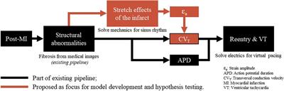
Our hypothesis is that a link between recurring fiber-strain amplitudes and CVT can be of importance to the development of substrate-based VT, as fiber-strains during the cardiac cycle are affected by stiff fibrosis. We expect that via strain amplitudes, the presence of the infarct affects CVT not only in the infarct core and border zone (BZ), as implemented in conventional heart models, but also in remote tissue parts where mechanics is impaired due to the adjacent structural infarction. Therefore, in this study, we propose a phenomenological model of the relation between fiber-strain amplitude and CVT. To test our hypothesis, the phenomenological model proposed is implemented in an existing pipeline (Figure 1). The effects of our hypothesis on electrophysiology simulation outcomes are analyzed in terms of CVT distributions, repolarization time gradients, and virtual stress test results. Finally, the sensitivity of repolarization time gradients to the definition of the strain-CVT relation is explored as well.

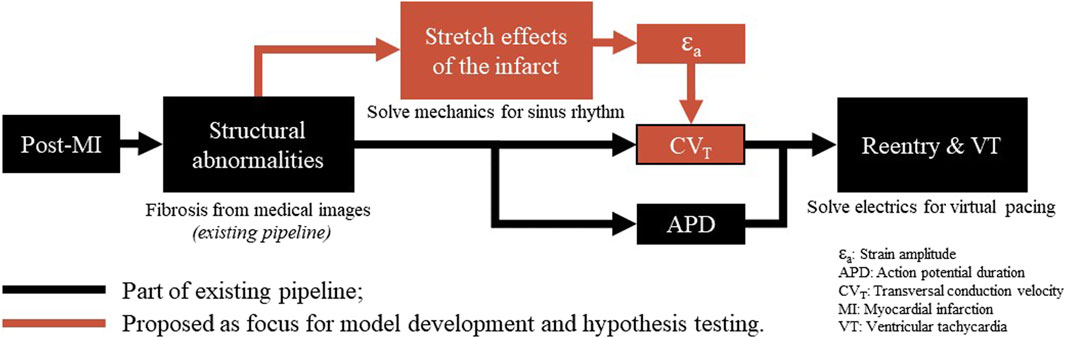
Figure 1. Overview of a virtual-heart model to simulate VT. In the current methods (black), the effect of the structural infarct area is taken into account by altering ion channel properties, which affect the action potential duration, and by reducing CVT. In this paper, an extension (red) is proposed to include strain-induced remodeling of CVT as well, which is important for VT risk evolvement over time. Finally, for both models with and without extension, a virtual stress test is performed in an attempt to induce VT.

The simulations are performed on a truncated ellipsoidal geometry with a rule-based myofiber field, which represents an idealized LV (Bovendeerd et al., 2009). The wall and cavity volumes are set to 136 and 44 mL. In the ellipsoid, two infarct geometries are considered, where the infarct core extends from 14% to 51% of the ventricle height (Figure 2A). A 100%-transmural core enclosed by a 9 mm thick BZ is implemented to ensure the induction of VTs, as it is known that larger BZs give higher risk for VT. Secondly, an endocardial 67%-transmural core with a 9 mm thick BZ is implemented to investigate whether the extension has the same effect for a non-transmural infarct. The total infarct volumes, including core and BZ, are 15 mL and 11 mL respectively.

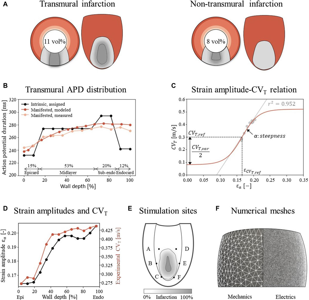
Figure 2. (A) Visualization of infarct and BZ in a short axis cross section at ¼ height of the LV, and in a long axis epicardial view. In shades of red, the distribution of different myocardial layers is visualized, as given in subfigure (B) In gray, two different combinations of infarct core and structural BZ geometries are schematically depicted, where the latter is a mixture of fibrotic and healthy tissue. The total infarct volume % of the LV is given for both situations. (B) For each myocardial layer, a different intrinsic APD is modeled by altering the Gks conductivities to mimic manifested APD measurements as presented by Poelzing et al. (Poelzing and Rosenbaum, 2004). (C) Eq. 2.4 (red) describes the phenomenological relation between fiber-strain amplitudes εa and CVT when fact is set to 1. Eq. 2.4 is fitted to a linear regression line through the combined data sets of subfigure D (gray). The meaning of the parameters is visualized in the figure, and corresponding values are given in Table 1. (D) Experimental CVT measurements as obtained from Poelzing et al. (red) ((Poelzing et al., 2004) and simulated strain amplitudes εax (black) over LV wall. (E) Visualization of six pacing sites at the endocardium. (F) Difference in mesh resolution for the mechanical (3 mm) and electrophysiological (500 μm) simulations.

The model of Janssens et al. is applied to simulate the mechanical behavior of a chronic infarct ventricle (Bovendeerd et al., 2009; Janssens et al., 2023). The material model and parameter values are copied from this study as well. A brief summary of their methods will be given in this section.

The myocardium is modeled as a non-linear, transversely isotropic, nearly-incompressible material. The Cauchy stress tensor is given by

This tensor is composed from two parts to account for both passive, σpas, and contractile active, σact, myocardial stresses. σact depends on the time t elapsed since cardiac activation, and on the length l of the contractile element. This active component is only present in parallel with the myofiber orientation e⇀f. To simulate a chronic infarct, the passive stress σpas is increased by changing the multiplication factor fpas from 1 to 10 in the infarct core to represent stiff fibrosis. Furthermore, the active component is eliminated by setting the multiplication factor fact to 0 to represent the loss of contractile myocytes in this area. To simulate the structural BZ, which is a mixture of infarct and healthy tissue, both fpas and fact values are linearly interpolated from the infarct core to the surrounding healthy tissue, where they are set to 1. The infarct size and geometry differ from those in Janssens et al., and are described in Sec. 2.1.

The ventricle is coupled to a 0D closed-loop lumped parameter model, which represents the circulatory system. Finally, the equation of conservation of momentum is solved:

Rigid body motion is suppressed by restricting the in-plane solution of basal nodes to its nullspace, which suppresses the average rotation about the long axis as well, and by constraining the base in the out-of-plane direction. The endocardial surface is subject to a uniform pressure. During isovolumetric contraction and relaxation, this pressure is determined such that mechanical equilibrium is obtained at a constant LV volume. The pressure during filling and ejection is computed from the interaction with the circulatory system. The simulated cardiac cycle is initiated by homogeneous activation of the myocardium. Strains are computed by using the LV geometry at t = 0 as reference, and fiber-strain amplitudes are defined as the difference between the local maximum and minimum logarithmic fiber-strain as experienced during the computed cardiac cycle.

Following the electrophysiology methods of Arevalo et al. (Arevalo et al., 2016), the monodomain equation is used which models cardiac tissue as excitable medium, with diffusion and local excitation of membrane voltage:

σm is the conductivity tensor describing the effective voltage diffusion through the tissue, Vm the membrane voltage which is solved for, β the membrane surface area-to-volume ratio, Cm the membrane capacitance, Iion the ionic model which describes the total transmembrane current, w the ionic variables, and Iext is an external stimulus current which can be applied. A zero transmembrane potential flux is imposed on the domain boundary, assuming there is no current flowing into or out of the domain. In this study, β is set to 0.14 μm-1, Cm to 1 μF/cm2, and Iextt to 40 μA/cm2 during the delivery of stimuli.

For Iion, the Ten Tusscher ionic model for human ventricular myocytes is used (Ten Tusscher and Panfilov, 2006). The structural BZ is simulated by altering peak conductivities which are kept constant over the whole BZ: for the sodium current (−62%), L-type calcium current (−69%), and potassium currents Gkr (−70%) and Gks (−80%) (Arevalo et al., 2016). This causes an elongation in action potential duration (APD), decreased upstroke velocity and decreased peak amplitude compared to the healthy modeled myocytes. In contrast to the model of Arevalo et al., an intrinsic transmural gradient in APDs is implemented in the remote tissue by altering the peak Gks potassium current in the endocardium (+110%), sub-endocardium (−5%), midlayer (+30%), and epicardium (+145%), yielding intrinsic APDs of 242, 294, 274, and 232 ms respectively when paced with a basic cycle length of 600 ms in single cell simulations. In tissue simulations, this manifests APDs that gradually increase from 238 ms at the epicardium to 282 ms at the endocardium (Figure 2B), which is in agreement with measurements of canine APDs (Poelzing and Rosenbaum, 2004). The gradual increase and maximum difference of 44 ms corresponds with measurements in healthy areas of human hearts (Boukens et al., 2015; Srinivasan et al., 2019). Those manifested (tissue) APDs differ from the intrinsic (isolated cell) APDs due to cell-to-cell communication, also called the electrotonic coupling of cells. The thicknesses of the 4 transmural layers are based upon methods in (Franzone et al., 2006). Those layers and the APD distributions are visualized in Figure 2B.

To simulate electrical pulse propagation, the along-fiber conductivity value for σm is determined to match a CV along the myofibers of 0.6 m/s in remote and BZ tissue. The conductivity is set to 0 in all directions in the infarct core. In the reference model, the methods of Arevalo et al. are followed further by setting CVT (thus in sheet and normal direction) to 0.3 m/s in remote tissue. In the structural BZ, CVT is set to 0.08 m/s and kept constant to represent the effect of a 90% decrease in transverse conductivity (Arevalo et al., 2016). In our extended model, the implementation of CVT deviates from that of Arevalo et al., as explained in the next section.

This is a sigmoidal relation (Figure 2C) where the CVT boundaries are set within a physiological range for surviving myocardial tissue. These boundaries are controlled by the allowed variability, CVT,var, around the basic velocity CVT,ref, which is chosen such that the minimum velocity matches the minimum in the reference model of 0.08 m/s. The function will return 1 if the local strain amplitude equals εCVT,ref, which will result in a CVT of CVT,ref (0.3 m/s) when using Eq. 2.4. The steepness α and shift εCVT,ref of the relation are chosen to match CVT sensitivity to strain. Their values are determined from combining a canine CVT dataset from literature (Poelzing et al., 2004) with strain amplitudes εa obtained from a simulation of healthy LV mechanics (Sec. 2.2). εa and CVT are both transmurally sampled in a 2 cm thick slice at the equator of the LV and increase over the wall depth from epi-to endocardium (Figure 2D). This positive correlation (r2 = 0.952) is reflected in a positive slope in Eq. (2.5) through α. All parameter values are given in Table 1. For both the reference and extended model CVT is zero in the infarct core, but for the extended model, CVT is expected to be more heterogeneous and to extend beyond the structural BZ into the functional BZ with impaired mechanics, which cannot be detected from contrast enhanced images. To determine CVT values in the electrophysiology model, a weak coupling between the models of mechanics and electrophysiology is established. This is done by obtaining strain amplitudes εa and infarct density fact from the model of mechanics, which are then used in Eq. 2.4.

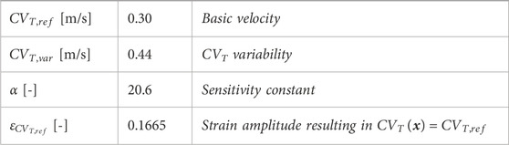
Table 1. Parameter values in Eq. 2.4 and Eq. 2.5 to describe the relation between fiber-strain amplitude and CVT, visualized in Figure 2C.

To evaluate VT risk, a virtual stress test is performed. In such a test, electrical stimuli are applied at six different sites, A through F, around the BZ at the endocardium (Figure 2E) (Kruithof et al., 2021). First, the Ten Tusscher cell model was stimulated 500 times prior to tissue simulations to reach steady-state. The resulting states of gating variables are given as input for the tissue simulations. For these tissue simulations, at each defined site, six stimuli (S1) with a cycle length of 600 ms are applied, followed by a premature stimulus (S2). To explore the vulnerable window in which VTs can be induced, a range in S2 timings with 5 ms increments from earliest electrical capture to 15 ms after the latest induced VT is simulated, resulting in a range from 320 to 370 ms. Each stimulus has a duration of 2 ms, an amplitude of 40 μA/cm2 and is applied to a tissue area with a diameter of 3 mm.

Unstructured finite-element tetrahedral meshes are generated with an average resolution of 3 mm and 500 μm for the mechanics and electrophysiology model respectively (Figure 2F). Mechanics simulations are performed in FEniCS with timesteps of 2 ms (fenicsproject.org). The displacement field is represented by quadratic Lagrangian basis functions, corresponding to a system of 106,852 degrees of freedom. Electrophysiology simulations are performed in the CARP framework with timesteps of 20 μs (opencarp.org). The membrane voltage potential is approximated by linear Lagrangian basis functions, corresponding to 108,2784 degrees of freedom. To incorporate mechanical results into the electrophysiology simulation, fiber-strain amplitudes are linearly interpolated from the lower resolution mechanics mesh to the higher resolution electrophysiology mesh. From these interpolated strain-amplitudes, CVT values are obtained through Eq. 2.4 and discretized in 9 levels from which the center values are imposed to the extended electrophysiology model using the methods of Costa et al. (Costa et al., 2013).

The effect of strain-induced CVT remodeling on the electrophysiological simulation outcomes is explored for the two infarct cases as depicted in Figure 2A. For each case, one mechanics cardiac cycle was simulated. Fiber-strain amplitudes from these simulations were used in the extended model to modify the distribution of CVT. Virtual stress test simulations from Sec. 2.2.3 are performed for both the reference and extended model to assess the effect of strain-dependent CVT.

To investigate the sensitivity of the results to the parameter settings of the novel strain amplitude-CVT relation, the values of α (steepness) and εCVT,ref (shift) were varied with respect to the baseline values as presented in Table 1 α was set to 50%, 70%, 100%, 150% and 250% compared to the default value. εCVT,ref was set to 122%, 111%, 100%, 89%, and 78%. This results in even distributions of strain amplitude-CVT curves as shown in the top row of Figure 7, which are applied to the transmural infarct case. For datasets with overall higher measured strains (large εCVT,ref), typically a lower sensitivity to variations in strain (small α) is expected. Therefore, when both parameters are varied, only smaller values for α are considered for larger values in εCVT,ref.

The simulation results are analyzed in terms of the spatial repolarization time gradients (RTG) map. This map is created for the last S1 stimulus in the simulation, where repolarization time is defined as the moment at which the membrane voltage repolarized to −70 mV. From these RTG maps, RTGvol and RTGmean metrics are extracted where RTGvol [ml] represents the tissue volume with gradients ≥10 ms/mm, which are critical for conduction block (Restivo et al., 1990). RTGmean [ms/mm] indicates the mean RTG value within this volume with RTGs above 10 ms/mm. These metrics are computed for all performed experiments, such that the effects of mechanical feedback and parameter variability on RTG can be explored. The RTG metrics during baseline rhythm are an indication for VT risk (Cluitmans et al., 2021), and only require S1 stimuli. For the sensitivity test, these metrics are computed for one pacing site only (site A in Figure 2E) to save computational costs.

For the virtual stress test simulations, all six pacing sites are used and S2 stimuli are applied as well. The results are captured in vulnerable windows. These windows define for each pacing site and S1-S2 interval whether VT was induced or not. Here, VT is defined as electrical activity sustained for at least 800 ms after S2. In case of occurrence of VT, exit points are defined as the location with earliest second activation time, counted from the start of S2 sustained for at least 800 ms after S2. In case of occurrence of VT, exit points are defined as the location with earliest second activation time, counted from the start of S2.

For the simulations of cardiac mechanics, PV-loops are created to capture the global function of the healthy and infarcted ventricles (Figure 3). Stroke volume and ejection fraction for the healthy case are 68 mL and 61% respectively. For the transmural and non-transmural infarcts, this reduced to 57 mL and 55%, and 58 mL and 56% respectively.

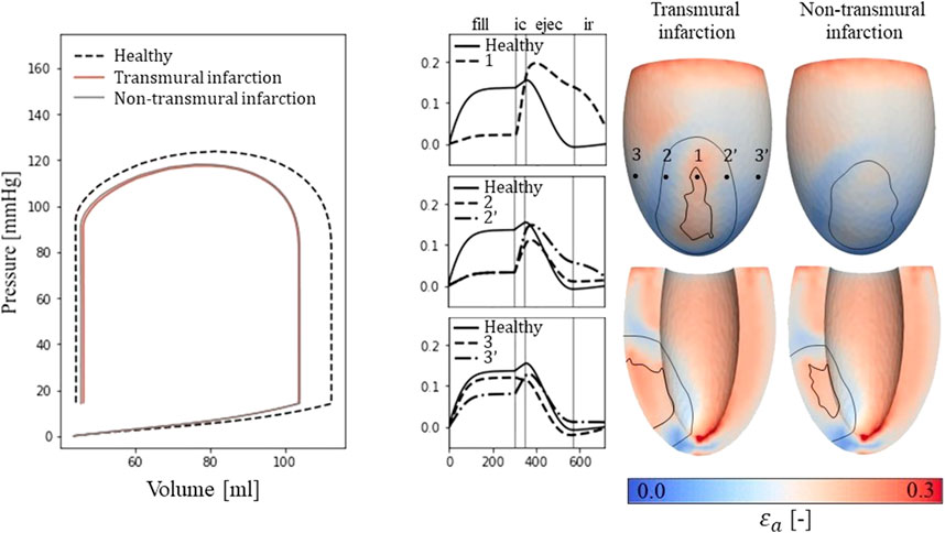
Figure 3. Left: PV-loops as simulated for the healthy LV and the implemented infarcts. Right: myofiber-strain traces during the cardiac cycle where the filling, isovolumetric contraction, ejection, and isovolumetric relaxation phases are indicated with vertical lines. Next to it, spatial distributions of strain amplitudes are given for the infarct cases with an epicardial (top row) and a cross-section view (second row) in which the structural infarct core and border zone are indicated with black lines.

Epicardial fiber-strain traces over time for a healthy case, at the infarct core, the outer BZ, and remote close to the BZ are given in Figure 3 (right-side). For the healthy case, myofiber strain rises during filling and decreases during the ejection phase. At the infarct core (location 1), the fiber-strain shows less increase during filling due to the increased passive stiffness in this area. However, the lack of contractility in this area results in tissue bulging (stretch) during ejection, increasing the fiber-strain during this phase. Therefore, strain amplitudes are still high in the infarct core. For the outer structural BZ (location 2 and 2′), strain during filling is reduced as well as this region is adjacent to the stiff core. Bulging during ejection is less compared to that in the infarct core as active contractile function is mostly retained in the outer BZ, resulting in low amplitudes in and around this region. Finally, in remote tissue close to the BZ (location 3 and 3’), strain traces become more similar to those of the healthy case. Asymmetry in strain results left and right to the infarct is induced by different fiber orientations in those regions relative to the infarct. Overall, strain amplitude is lower at the epicardium compared to the endocardium, in the structural BZ of the infarct, and in parts of remote tissue closely located to the structural BZ.

From the distributions of strain amplitude (εa and scar density (fact, the LV distributions of CVT are created (Eq. 2.4) for the healthy and two infarct cases. A wider distribution of CVT values is observed for the infarct cases compared to the healthy case (histogram Figure 4), as both εa and fact are affected by infarction. For the healthy case, all velocities are within range of 0.20 and 0.49 m/s, where the majority is between 0.26 and 0.43 m/s. For the infarct case, the majority is still within the same range, but conduction slowing induced velocities below 0.20 m/s as well.

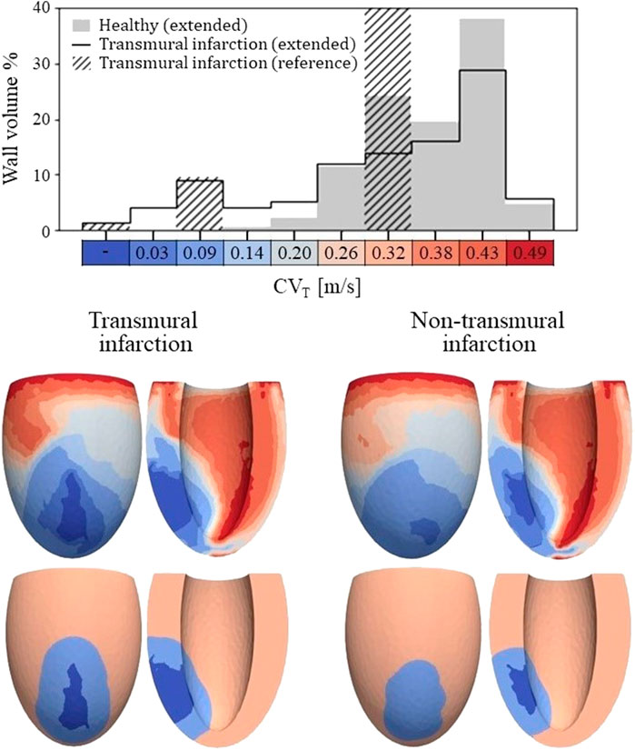
Figure 4. Top: Histogram of CVT values for the healthy and transmural infarct case as obtained with the extended model. The majority of the tissue in the extended models has a CVT in the range of 0.26–0.43 m/s. For the infarct case, velocities below 0.2 m/s are observed, which are not present for the healthy case. Furthermore, CVT for the reference model is given as well, in which CVT is divided over three velocities to represent completely non-viable (first bar), BZ (third bar) and remote tissue (seventh bar). For this reference model, a velocity of 0.3 m/s is assigned to tissue remote from the infarct, which covers 89% of the wall volume (out of frame in the histogram shown). Bottom: Spatial CVT distributions over the LV for the two chronic infarcts, for the extended (top row) and reference model (bottom row). The same discretization and colors are used as for the histogram above.

The spatial distributions of CVT are shown in the lower half of Figure 4. For both reference (bottom row) and extended (top row) models, conduction slowing is mainly localized at the infarct region. However, for the extended models, this is not limited to the structural BZ but extends to remote parts close to the infarct as well. These regions can be described as functional BZ as they have impaired mechanics due to their connection to the infarct area. Through the model extension, the tissue volume with severe conduction slowing (CVT ≤ 0.1 m/s) increased from 13.0 to 17.5 mL (+35%) for the transmural infarct case. For the non-transmural infarct case, this increased from 10.6 to 17.6 mL (+66%). Furthermore, CVT heterogeneity is present in far remote tissue, where higher values are located towards the endocardium, and rapid CVT changes are present at the apex.

A total of 24 (2*12 settings) RTG maps were created, 2 CVT distributions (reference and extended) for the 2 infarct cases with 6 stimulus sites each. We found that largest RTG values are clustered at the boundary of the structural BZ, in which a prolonged APD was implemented. The mechanics-extension further enhances these high RTG values at the structural BZ boundary (Figure 5, left).

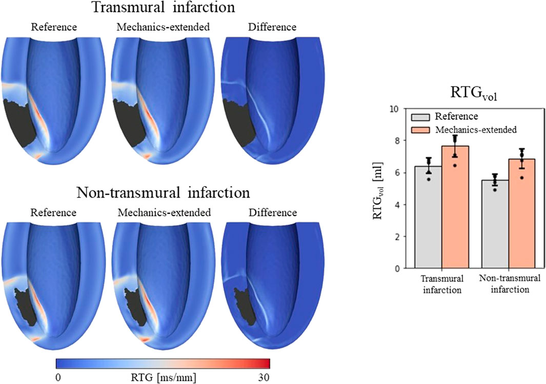
Figure 5. Left: repolarization time gradient maps for the reference model, extended model, and the difference (mechanics-extended minus reference). The extended model further highlights the high gradients on the boundary of the ionic-remodeled border zone. Right: RTGvol and RTGmean per pacing site (dots), with their average values (color bars) and standard deviations (black bars) for both the reference and extended models.

RTGvol and RTGmean values with their average and standard deviations across the 6 stimulation sites are presented in Figure 5 (right-side). The mechanics extension causes RTGvol to increase for all 18 simulation settings. For both infarct cases, this increase in RTGvol is on average 1.3 mL. The mechanics extension has minimal effect on RTGmean, which is similar for reference and mechanics-extended simulations, and remains between 12.7 and 14.0 ms/mm for all simulations. RTGmean increased with 0.09 ms/mm for the transmural cases, and with 0.26 ms/mm for the non-tranmsural infarct case. Overall, strain-induced remodeling increased both the volume with severe conduction slowing and RTG the most (dangerous) for the non-transmural infarct case. For a more detailed insight in the effect of the extension on RTG, RTG histograms for the transmural infarct case are given in Supplementary Appendix A.

Vulnerable windows for both the reference and extended models are given in Figure 6 (middle). The mechanics-extension has several effects. For the transmural infarct, it more than doubled the vulnerable window width. Importantly, the three VTs as induced in the reference model (labeled X, Y and Z in Figure 6) could be replicated. Their exit sites covered a larger area (orange lines in Figure 6, right-side) compared to the reference results. Additionally, two novel VT patterns (U and V) could be induced. A more detailed analysis showed that the increased inducibility in the extended model was caused by an elongated line of conduction block compared to the reference, due to the enhanced RTGs on the structural BZ boundary. This, together with the additional conduction slowing adjacent to the structural BZ, allowed VT to be more easily sustained. The membrane voltage plot left in Figure 6 demonstrates this finding: the reentrant pathway is not sustained in the reference model, as the tissue was not ready for re-activation when the wavefront arrived too early, in contrast to the extended model due to a slightly longer cycle time.

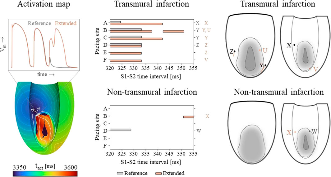
Figure 6. Left: an example of an VT activation times map which shows that VT inducibility can differ for the two models, especially when the effect of the S2 stimulus is on de edge between propagation (white arrow) or conduction block (white block). Middle: vulnerable windows are given with pacing sites A through F on the vertical and S1-S2 time intervals [ms] on the horizontal axis. Color coding indicates whether VT was induced for the reference (gray) or the mechanics-extended model (orange). Characters (U-Z) are used to indicate which windows showed the same VTs. Right: Exit points for each VT pattern are visualized in a schematic representation of the epicardium and endocardium. The assigned characters correspond to those next to the vulnerable windows, and are colored orange if they appeared in the extended model only.

Despite its high RTG metrics, only small vulnerable windows are present for the non-transmural infarct case (Figure 6, middle). The induced VT patterns differ completely between the reference and extended model. However, their small inducibility windows (5 ms) make them clinically irrelevant.

The α and εCVT,ref parameters of the strain amplitude-CVT model (Eq. 2.4; Eq. 2.5) were varied to perform a sensitivity test on the transmural infarct case. This resulted in steepness and horizontal shift variations of the strain amplitude-CVT relational curve as shown in the top row of Figure 7. For each setting, a simulation is performed resulting in a total of 13 RTG maps which are analyzed in terms of RTGvol and RTGmean. Within the tested range, the maximal variation in RTGvol (second row of Figure 7) is smaller for altering α (0.9 mL) or εCVT,ref (0.6 mL) than for altering pacing sites (1.7 mL, right side Figure 5: mechanics-extended, transmural infarction). The variations in RTGmean are minimal. Finally, with the simultaneous increase of α and decrease of εCVT,ref, variability in RTGvol (0.29 mL) and RTGmean (0.2 ms/mm) is smallest as the curves overlap in the low range of CVT, critical for cell-uncoupling and thus RTG. This overlap is also present in histograms of critical RTGs, from which a complete overview is given in Supplementary Appenidx B.

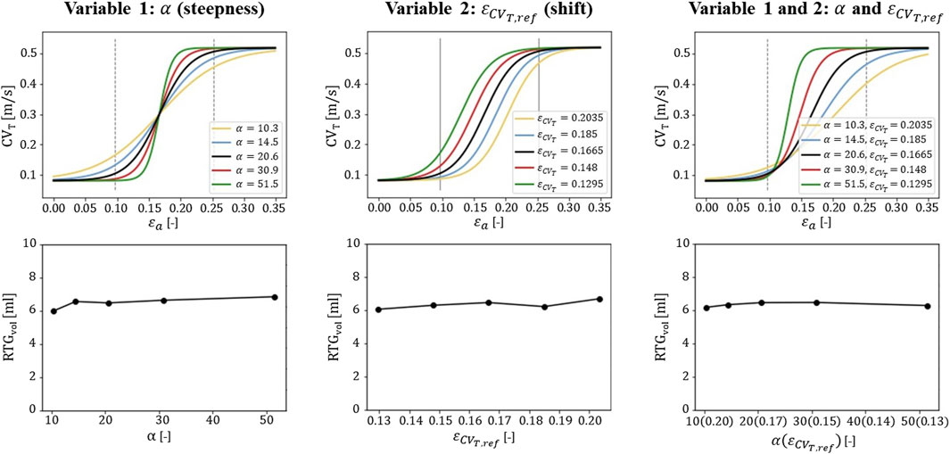
Figure 7. Sensitivity testing of the gεax function. The α and εCVT,ref parameters are adjusted to obtain homogeneous increments in steepness and shifts of the curve (top row). The corresponding effects on RTGvol is shown for one pacing site (second row). The central values for α and εCVT,ref (black lines in the top row) are used as default for the stress test simulations (Table 1) for which six pacing sites are used.

To include the effect of mechanical tissue load, we introduced several modifications to our reference electrophysiology methods. First, in the reference model, CVT is altered in the structural BZ based on measurements in canine infarcts (Yao et al., 2003). Supported by cultured cell experiments, we proposed a phenomenological model in which CVT is altered by recurring strain amplitudes, on top of the effect of structural abnormalities. We found a strong positive correlation (r2 = 0.952) between experimental CVT (Poelzing et al., 2004) and simulated myofiber strain amplitude, as they were both lower at the epicardium and higher in the last 60% towards the endocardium. We fitted the model on this correlation, by setting the central CVT to 0.3 m/s as is done conventionally, around which CVT varies due to the effects of strain. This adaptation results in different CVT values for infarct and healthy regions as strain modulates around the stiff infarct.

Second, the effect of fibrotic density on CVT is modelled as a continuous linear relation, instead of the discrete 3-level relation assumed in conventional models. In this way, the highest fibrotic density naturally results in no electrical activity in the non-viable infarct core. Additionally, the spatial CVT distribution is more heterogeneous as it results from the combined effects of fibrosis and fiber-strain amplitudes. These amplitudes are, for example, not constant over the wall depth, and are modulated nearby the stiff infarct. The CVT distribution is therefore discretized in 10 levels instead of the aforementioned 3 (core, structural BZ, and remote) in the reference model.

Thirdly, in order to follow the Poelzing data used in the relationship between experimental CVT and strain, we introduced in our model the transmural APD gradient present in those experimental canine data too. The presence of such transmural APD gradients in human data has been a topic of discussion (Boukens et al., 2015). For completeness, we have performed simulations without the transmural APD gradient too (Supplementary Appendix A). Here we implemented a homogeneous APD (287 ms when paced with 600 ms intervals) over the wall depth. For these simulations, RTGs were lower than for the simulations with transmural APD gradient, and no VTs could be induced. This might be caused by the smaller difference in APD between remote and border zone tissue in this model. Moreover, the occurrence of VT is a binary ‘all-or-nothing’ response, sensitive to various modeling choices. Introducing the effect of strain on CVT might result in VTs in more critical cases. However, the impact of mechanics on electrophysiology substrate is similar under both conditions (with and without transmural APD gradient), enhancing RTGs on the border of the infarct area.

Fourth, we apply a weak coupling between the model of mechanics and electrophysiology. This is motivated from the long time-scale of conduction remodeling observed in cultured cell experiments. This remodeling took a few hours of applied pulsatile stretch, and persisted several hours after the stretch was removed. We assumed that recurring ‘pulsatile’ strains are mimicked during hours of sinus rhythm, which will induce remodeling of CVT. These effects would persist long enough to remain in the short timeframe during which stress test pacing is applied. Additionally, the period of pacing is too short to induce further remodeling. It was therefore sufficient to only simulate mechanics during sinus rhythm, from which the results are used to define a static distribution of CVT. The numerical un