Starfysh modelModel overview

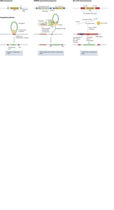
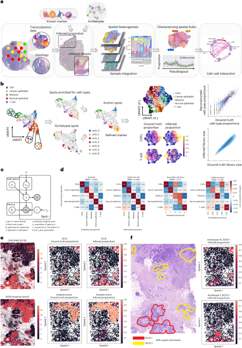
Deep generative models parameterized by neural networks have proven effective in analyzing single-cell RNA expression data (scvi-tools19, scVI20, totalVI21, scArches22, trVAE23, scANVI24, MrVI25 and so on). However, the presence of multiple cell types in each spot in ST data makes it difficult for these models to disentangle cell type-specific features. To overcome this limitation, Starfysh introduces a generative model with a special variational family that is structured to model the presence of multiple cell states per spot in ST data. The Starfysh generative model leverages gene set signatures (either existing signatures or signatures computed with archetypal analysis) as an empirical prior to help disentangle cell types72. We first detail the generative model of Starfysh and then introduce its structured variational family.

Starfysh generative process

Starfysh models the vectors of gene expression \(_\in }}^\) (with G the number of observed genes) for each spot i with a generative model. The generative model (Fig. 1c) is parameterized by K, representing the expected number of cell states in the data. The determination of K can be automated through archetypal analysis beforehand, or an expert can provide guidance on the K most important cell states in the sample. Each cell state k ∈ [K] is characterized by a low-dimensional latent variable, \(_\in }}^\) (with D defaulting to ten dimensions), capturing the specific mechanisms underlying that cell state. Moreover, each cell state k has a scalar variable, σk > 0, indicating its variability and heterogeneity.

Subsequently, Starfysh models each spot i with a specific low-dimensional representation zi. In the context of single-cell data, each cell state k would usually be represented by a low-dimensional vector z centered around uk, with a standard deviation of σk. However, for ST data, where each spot captures a mixture of cells with different cell states, Starfysh associates each spot i with a proportion vector, ck ∈ ΔK, representing the proportions of each cell state in that spot. Starfysh then constructs the low-dimensional representation zi with a mixture distribution that combines the cell state proportions ci and the cell state-specific representations uk: \(_|_,\,\sigma \sim N(__}_,__}_)\).

Following this, zi is transformed using a neural network f to obtain the normalized mean expression of each gene for spot i, which is further scaled by the library size li. The observed raw transcript count xig for gene g in spot i is then sampled from a negative binomial distribution centered around the upscaled mean.

Cell state proportions, ci, are also considered as random variables with a carefully crafted prior. Each cell state k ∈ [K] needs to be associated with a preliminary gene set signature, sk, which can be provided by the user or automatically discovered through archetypal analysis. By calculating the signature scores in each spot, denoted as A(xi, sk), Starfysh establishes a prior distribution over the cell state proportions in each spot. Specifically, the proportions of cell states ci are sampled from a Dirichlet distribution with a prior parameter α[A(xi, sk)]k∈[K]. For instance, if spot i highly expresses known marker genes for cell state k, then a larger value of A(xi, sk) will favor the probability of allocating cell state k for spot i according to the empirical Dirichlet prior parameter. The parameter α modulates the prior strength and represents the belief in the signature gene sets: a larger value corresponds to a stronger prior, while a smaller value results in a less constraining prior.

The generative model is defined as \(p(u,,,,)=_^p(_)_^\)\(p(_)p(_|_,u)p(_)p(_|_,_)\), with

p(uk) = Normal (0, 10ID)

p(ci; α, A) = Dirichlet (α⋅A), where α controls the prior strength on the signature scores A.

p(zi|ci, u; σ) = \(}(\sum __}_,\sum __}_)\), where the parameters σk represent cell state-specific heterogeneity.

\(p(_}\widetilde_})=}(\widetilde_},1)\), where \(\widetilde_}\) is the locally averaged library size observed in spot i’s spatial neighborhood.

p(xi|zi, li) = \(_^p\left(_}}_,_\right)\,\)

p(xig|li, zi; θg, f) = NegativeBinomial (lif(zi), θg), where θg denotes gene-specific dispersions and f is a neural network with a softmax output.

In the generative process, the parameters \(A,\alpha ,\widetilde_}\) are fixed. The prior strength α is set by default to 50. Robustness analysis on α demonstrates that the model consistently outperforms the signature prior given a reasonable range (α ≥ 1) (Supplementary Fig. 2c). The optimal choice of the prior strength term depends on the specific dataset and markers. The locally averaged library size is computed as \(\widetilde_}=\frac_|}\,\sum __}_\;_}\), where Ni is the set of spots physically located adjacent to spot i and also includes i. The cell state heterogeneities σk are initialized as 1, and the gene dispersions θg are initialized at random. Finally, the neural network f has by default one linear layer followed by a softmax. σk, θg and f are all learned during the inference.

Integration with histology images

Although histology hematoxylin-and-eosin (H&E) images are usually provided along with ST data (for example, the commercial Visium platform), current methods fail to use such modality in deconvolving cell types. Histology, however, provides useful information about morphology, tissue structure, cell density and spatial dependency of cells. Integrating histology and transcriptomes in a joint model is challenging, as the two data modalities are very different: the genome-level transcripts are high-dimensional vectors, whereas the histology data consist of multichannel images. Thus, it is essential to address the mismatch of these two types of data while preserving cell type-specific information of gene expression and cell morphology-specific information of histology images. The integrative approach in Starfysh is formulated with a deep variational information bottleneck26.

The original H&E images are first normalized to [0, 1] per channel. The alignment between H&E images and ST spot i produces the histology image patches \(_\in }}^\) (with P as the side length of the patch and C as the number of image channels, for example, C = 3 for RGB images and C = 1 for grayscale images). We set P = 26 by default to approximate the number of pixels surrounding each spot. The image patch yi is then flattened in the Starfysh model and assumed to be generated from the same latent variable zi that informs gene expression (Fig. 1c and Supplementary Fig. 1a) with a distribution p(yi|zi) parameterized by two neural networks gμ, gσ, for mean and variance of distribution for yi, respectively. Both consist of a linear layer followed by a batch normalization layer. They define:

$$p\left(\;_}_\right)=}\left(\;_(_),_(_)\right).$$

Construction of the empirical prior

For cell states expected to reside in the tissue, Starfysh first filters out marker genes that are either unavailable in the ST data or not expressed in any spots to obtain binary variable \(_\in }}^\), k = . Next, two priors are calculated before running Starfysh, including a prior for the cell state proportions that reflects their spot enrichment and a prior for the library size:

1.

Prior for the cell type proportion:

A(xi, sk) is defined as the enrichment score74 of the marker genes for cell state k at spot i. The score is first calculated with the Scanpy function ‘scanpy.tl.score_genes’, which computes the marker genes’ average expression and subtracts from it the average expression of a reference gene set G′ randomly sampled from binned expressions: \(^}}(_,_)=\frac_}_\;_}\cdot _}-\frac}_}_}\). We further transformed the scores using the function ReLU(x) = max(0, x) to ensure the positive constraints of Dirichlet parameters and make them comparable across spots (with ϵ defaulting as 1 × 10−5):

$$A(_,_)=}(^}}(_,_))+\epsilon$$

$$A(_,_)=\frac_,_)}_A(_,_)}.$$

For each cell state, the prior assigns unique enrichment scores across all spots, and we thus can define the anchor spots \(R\in }}^\) specifying the ranking of each spot i based the enrichment score \(A(:,)\) for each state \(k\), which can be updated with archetypal analysis detailed below.

2.

Prior for the library size:

Starfysh also considers the spatial dependency of spots when generating the prior for library size. \(\widetilde_}=\frac_|}\,\sum __}__}\), where \(_\) is the set of spots physically located around the spot i, which includes all spots j such that \(|_}-_| < w\), where w is an adjustable parameter for window size (default set to 3). \(_\) is the spatial coordinates for spot i.

Archetypal analysis

Marker genes that represent cell states may be context dependent or unknown. To address these limitations and improve the characterization of tissue-dependent cell states, we developed a geometric preprocessing step, leveraging archetypal analysis75, to refine marker genes and identify new cell states.

Archetypal analysis fits a convex polytope to the observed data, finding the prototypes (archetypes) that are most adjacent to the extrema of the data manifold in high dimension. Previous works76,77,78 have applied archetypal analysis to scRNA-seq data to characterize meaningful cell types. In the context of ST, we hypothesize that the archetypes are closest to the purest spots that contain only one or the fewest number of cell states, while the rest of the spots are modeled as the mixture of the archetypes.

We applied the PCHA algorithm79 to find archetypes that best approximate the ‘extrema’ spots on a low-dimensional manifold. Specifically, let \(\hat\in }}^\) be the normalized spot (S) by gene (G) expression from the original spatial count matrix. We further selected the first P = 30 principal components (\(\in }}^\,\)) to denoise the data. We denote matrices \(W\in }}^,\in }}^\) and \(H=\in }}^\), where D represents the number of archetypes. The algorithm optimizes the parameters of W and B alternately, minimizing \( -WH\Vert }^= -WBX \Vert }^\) subject to \(_ > 0\;\&\; _^_=1\) and \(_ > 0\;\&\; _^_=1\), where S spot counts and D archetypes are convex combinations of each other74. We applied Fisher separability analysis80 to infer the intrinsic dimension as its lower bound and iterated through different K values until the explained variance converges. We also implemented a hierarchical structure to fine tune the archetypes’ granularity with a resolution parameter r (ref. 81) (default set to 100). For archetype ai, i ∈ 2,…, D, if it resides within a Euclidean distance of r from any archetype aj, j ∈ 1,…, i − 1, we merge ai with the closest aj. The archetypes distant from each other are kept after the shrinkage iteration and used in subsequent steps.

We define archetypal communities as the r-nearest neighbors (same as the resolution parameter) to each archetype by constructing D clusters. Next, for each cluster i, we identify the top 30 marker genes by performing a Wilcoxon rank-sum test between in-group and out-of-group spots with Scanpy82. We then refine cell state markers by assigning archetypal communities to the closest cell states. First, we align D archetypal communities with the best one-to-one matched K cell states with stable marriage matching83 and then append the archetypal marker genes to the given cell state. Next, we update the anchor spots according to the updated gene list. Alternatively, to find new cell states, we rank the archetypal clusters from the most distant to the least distant to the anchor spots of known cell states, and the archetypal clusters distant from all anchor spots represent potential new states for further study.

The overall archetypal analysis algorithm in Starfysh is summarized as follows:

1.

Estimate the intrinsic dimension of the count matrix, and find k archetypes that identify the hypothesized purest spots.

2.

Find the N-nearest neighbors of each archetype, and construct archetypal communities.

3.

Find the most highly and differentially expressed genes for each archetypal community, and select the top n genes (default, n = 30) as the ‘archetypal marker genes’.

4.

If the signature gene sets are provided, align the archetypal communities to the best matched known cell types, update the signature genes by appending archetypal marker genes to the aligned cell type and recalculate the anchors.

5.

If the signature gene sets are absent, apply the archetypes and their corresponding marker genes as the signatures.

We found that archetypes alone are sufficient for disentangling major cell types but not fine-grained cell states (Supplementary Fig. 3e); however, when used as empirical priors to the deep generative model, they can guide the successful deconvolution of cell states (Supplementary Fig. 3a).

Starfysh structured variational inference

Starfysh uses variational inference to approximate the posterior. We first describe the inference procedure without integrating the histology variable yi. The posterior on variables uk (cell states representations) are approximated by mean-field distributions q(uk), while the posterior on the variables ci and li (cell state proportions and library size) are approximated by amortized mean-field distributions q(ci|xi) and q(li|xi). Next, for each spot i, we use a specially structured variational distribution q(zi|ci, xi) that uses cell state proportions to sample the latent variables zi. Because each spot contains multiple cell states with proportions ci, the structured variational distribution is assumed to decompose as a combination of cell state-specific terms (denoted by ζ(k, xi) for each cell state k), weighted by the proportion of cell states ci. The variational family factorizes in the form \(q(u,,,)=_^q(_)_^q(_|_)q(_|_)q(_|_,_\;)\), parametrized by new variational parameters mk and vk and neural networks λ, γ and ζ as follows:

$$\beginq(_) \, = \, }(_,_)\\ q(_}_) \, = \, }\Big(_(_),_(_)\Big)\\q(_}_}\,\alpha ) \, = \, }\Big(\alpha \cdot \gamma (_)\Big)\\q(_}_,_) \, = \, }\Big(__}\cdot _(k,_),__}\cdot _(k,_)\Big).\end$$

In summary, for each cell state k, the function ζ(k, xi) deconvolves the contribution of cell state k to the latent representation of zi. Each zi is a combination of the cell state contributions ζ(k, xi) weighted by the proportions ci. The cell state proportions are inferred with the neural network γ, which is guided toward the prior to match the cell type gene sets. The prior strength parameter α also premultiplies the neural network γ to obtain a posterior of similar strength, which helps for the gradient optimization.

Next, the standard variational inference that maximizes the evidence lower bound (ELBO) is performed84. The ELBO in our case can be written as:

$$\begin}\left(q\right) \, = \, \mathbb_}x)}\left[\log \frac}\alpha ,A,\widetilde,\sigma \right)}}x)}\right]\\ \qquad\qquad\;\,\, = \, \,\mathbb_\right)}[\log p(x}z,l\;)]\\ \qquad\qquad\qquad\, \, -\mathbb_\left[_}}\Big(q(,x)\| p(z}u,c}\sigma )\Big)\right]\\ \qquad\qquad\qquad\, \, -_}}\Big(q(}\alpha )}p(c}\alpha ,A)\Big)\\ \qquad\qquad\qquad\, \, -_}}\Big(q(l}x)}p(l}\widetilde)\Big)-_}}\Big(q(u)}p(u)\Big),\end$$

where DKL(p || q) is the Kullback–Leibler divergence between distribution p and q, defined as DKL(p || q) = ?p(x)[log p(x)/q(x)]. We find the q that maximizes the ELBO by running stochastic gradient descent.

Starfysh structured variational inference with histology integration

To integrate the histology in the inference method, we model the approximate posterior over the latent low-dimensional representation z with the PoE distributions (Supplementary Fig. 1a). For each spot i, we denote the view-specific encoders qθ1 (zi|ci, xi) and qθ2 (zi|yi) from the corresponding expression xi and image patch yi, respectively. The expression view \(__}(_|_,_)=}(_,_}^)\) is the same as described. For the histology view, zi is approximated by amortized mean-field distribution \(__}(_|\;_)=}(_,_}^)=}(_(_),_(_))\) with a single-layer neural network \(\xi\). For the joint latent variables \(_\), the posterior distribution q(zi|ci, xi, yi) is parameterized as a product of view-specific Gaussian distributions as described in the original method26:

$$_(_}_,_,_)=\frac_/_}^+_/_}^}_}^+1/_}^}.$$

The previous ELBO can be updated with this new variational approximation for the joint modeling of histology and transcriptome. We leverage the information bottleneck approach26 to optimize the joint ELBO as well as the view-specific marginal ELBOs through a single objective function \(}}_}}=}}_}}+a\cdot }}_}}\), where:

$$\begin\quad}}_}} \, = \, }(_)=__(z,l,c,u}x,y)}\log \frac}\sigma )}_(z,l,c,u}x,y)}\\\qquad\qquad= \, __(z}x,y)_(l}x)}\,\log p(x}z,l)+__(z}x,y)}\log p(y}z)\\ \qquad\quad\qquad-\,__(c}x)_(u)}_}}\Big(_(z}c,x,y)\| p(z}c,u}\sigma )\Big)\\ }}_}} \, = \, }(__})+}(__}).\end$$

The variational family for the joint objective function is factorized as \(_(z,,,,)=_(,)_(|\;)_()_(u)\). Hyperparameter a (set by default as 5) balances the weights between joint and view-specific objectives26. The expression view \(}(__})\) remains the same with above, and the histology view \(}(__})\) is written as:

$$\begin}(__}) \, = \, ___}(z}y)}\log \frac}\sigma )}__}(z}y)}\\\qquad\qquad\quad\,= \, ___}(z}y)}\log p(y}z)-___}\left(cy\right)__}\left(u\right)}_}}\left(__}(z}\;y)}p(z}u,c}\,\sigma )\right).\end$$

The same conditional prior p(z|c, u; σ) is applied across the joint and view-specific ELBOs. We find the \(\_,__},__}\}\) that maximize \(}}_}}\) by running stochastic gradient descent.

Starfysh implementation

The Starfysh model is implemented as a Python package using PyTorch85 with the Adam86 optimizer. The model by default is trained for 200 epochs with a learning rate at 0.001. During the training, the learning rate decays, guided by an exponential scheduler with the multiplicative factor set as 0.98. Kaiming initialization is applied to all neural network parameters. Hyperparameters are adjustable in the package.

Prediction of cell state-specific expression

To predict cell state-specific expression, we use the decoder in which the parameters have been learned and optimized by the variational inference. The proportion ci is adjusted to 1 for a specific cell state and 0 for other cell states. Reconstructed expression and histology are considered as cell state-specific expression and histology.

Integration of multiple samples

To effectively integrate multiple samples, Starfysh initially identifies anchors in each sample by combining spots enriched for cell types and archetypal communities. The gene markers for each sample are then updated based on the newly defined anchors. Subsequently, we aggregate the gene markers for each cell type across all samples. These updated markers are used to calculate priors for the cell state proportions when fitting to all samples simultaneously. Priors for library size are separately calculated for spots in each sample. Finally, transcriptomic counts along with their corresponding histological patches are incorporated as inputs to train an integrated model, synergizing data across samples.

Simulation of ST data

We construct our ST simulations using mixtures of scRNA-seq data previously collected from primary TNBC tumor tissues (CID44971_TNBC)18 with different levels of cell type granularities.

Spatially dependent simulation

To address spatial dependencies among neighboring spots, we adopt the pipeline from Cell2location8. Specifically, synthetic ST spots are defined on a 50 × 50-pixel grid. For the major cell type simulation, we select five cell types (CAFs, cancer epithelial cells, myeloid cells, normal epithelial cells, T cells) from the reference scRNA-seq data and simulate their spatial proportions with separate 2D Gaussian process models (Supplementary Fig. 2a). We further assign an expected library size for each spot with a γ distribution fitted from the real ST dataset, representing the spatial variation of capture rates among spots. For each spot, we then sample single-cell transcriptomes from the reference by searching for candidate cells with a library size closest to the expected library size. We follow the same procedure to generate another ten-cell type simulation with finer cell states: basal cells, inflammatory CAFs, myofibroblast CAFs, endothelial cells, immature PVL cells, central memory T cells, Treg cells, activated CD8+ T cells, memory B cells and plasmacytoid dendritic cells.

Simulation with paired histology images

We further generate pseudo-histology images paired with the aforementioned major cell type simulation to verify multimodel integration. Specifically, we design a supervised encoder–decoder neural network model (Supplementary Fig. 1c), with real ST expression as input and their histology images as output. First, the expression matrix is projected to a low-dimensional latent space with a ResNet18 encoder, and the histology image is reconstructed with a standard linear decoder with dimension transformation. Two thousand image patches and corresponding expression matrices were trained from 14 ST samples, and an extra 500 images patches were used for held-out validation. The learning rate was set as 0.001 with the Adam optimizer for training. Mean-squared loss was used to fit the predictions to the real ST images. The final paired synthetic histology images were generated by running the trained model.

Signature gene set retrieval in simulated data

For fair benchmarking not favoring Starfysh, we build the signature gene sets in an unbiased fashion by choosing the top 30 differentially expressed genes for each cell type (highest log (FC) scores) across 20 breast cancer scRNA-seq samples reported by Wu et al.18.

Benchmarking of Starfysh and comparison to other methods with simulated ST data

We benchmarked Starfysh against reference-based (DestVI, Cell2location, Tangram, BayesPrism) and reference-free (CARD, BayesTME, STdeconvolve) deconvolution methods with the aforementioned simulations. For the reference-based method, we used paired scRNA-seq data for sample TNBC sample CID44971 as the reference. For reference-free methods without inferred cell state annotations, we report the best alignment with the ground truth proportions upon permutation.

For each deconvolution, we trained Starfysh with three independent restarts and selected the model with the lowest \(}}_\). The variational mean q(cik|xi; α) is used as the inferred cell state proportions.

For BayesPrism, we followed the tutorial on the BayesPrism website: https://www.bayesprism.org/pages/tutorial_deconvolution. We subsetted the common protein-coding genes between the scRNA-seq and ST data with highly variable gene selection by default. We ran the BayesPrism Gibbs sampler ‘run.prism’ with four cores and extracted the updated cell type fractions θn for deconvolution.

For Cell2location, we followed the tutorial on the Cell2location website: https://cell2location.readthedocs.io/en/latest/notebooks/cell2location_tutorial.html. We trained the reference regression with 1,000 epochs and spatial mapping models with 10,000 epochs, in which ELBO losses were ensured. The normalized 5% quantile values of the posterior distribution \(}_}=\frac_}}__}}\) were used for deconvolution.

For DestVI, we followed the DestVI tutorial with default parameters at https://docs.scvi-tools.org/en/stable/tutorials/notebooks/DestVI_tutorial.html.

For Tangram, we followed the Tangram tutorial using default settings: https://github.com/broadinstitute/Tangram/blob/master/tutorial_tangram_with_squidpy.ipynb. We found the optimal alignment for scRNA-seq profiles with 1,000 epochs.

For CARD (reference free), we followed the CARD reference-free tutorial: https://yingma0107.github.io/CARD/documentation/04_CARD_Example.html. Default settings were used to generate cell type proportions (minCountGene = 100 and minCountSpot = 5).

BayesTME (reference free) deconvolves cell types with a hierarchical probabilistic model that corrects technical artifacts. We followed the official BayesTME tutorial with default parameters: https://github.com/tansey-lab/bayestme/blob/main/notebooks/deconvolution.ipynb.

For STdeconvolve (reference free), we followed the tutorial on the STdeconvolve website (https://jef.works/STdeconvolve/) and selected the top 1,000 overdispersed genes from the input matrix. We set the optimal number of cell types K to 5 and 10 for the major and fine cell type simulations, respectively. The predicted cell type proportions were obtained from the output ‘deconProp’.

Quantification of performance in deconvolution of cell types

The performance of each method was summarized by the RMSE and Jensen–Shannon divergence (JSD) against the ground truth to quantify per-spot accuracy (Supplementary Fig. 2d,e):

$$\begin}\left(_}^},_}^}}\right) \, = \, \sqrt\nolimits_^_}}^}-_}}^}}\right)}^}}\\\quad\; }\left(_}^},_}^}}\right) \, = \, \frac_}}\left(_}^}}_}^}}\right)+\frac_}}\left(_}^}}}_}^}\right),\end$$

where \(_}^},_}^}}\in ^\) represent the ground truth and predicted cell type compositions in spot i. We report the average RMSE across all spots as the overall performance for each method (Fig. 1d).

Benchmarking of Starfysh and comparison to other methods with real ST data

We further benchmarked Starfysh with reference-based (Cell2loation and BayesPrism) and reference-free (STdeconvolve) deconvolution methods on TNBC sample CID44971 ST data (Supplementary Fig. 3b–d). We calculated the correlation \(A\in }}^\) between the average expression of gene sets (normalized to sum to 1 per spot) (Supplementary Table 2) and the deconvolution profile for each cell state:

$$\begin_} & = & }\Big(_}^}},_}^}}\Big)\\ }_} & = & \frac__}\cdot _}}__}},_}^}}=\frac}_}}\nolimits_^}_}},\end$$

where \(_^}},_^}}\in }}^\) represent signature marker’s expression and deconvolution proportions for cell states k and l, respectively.

For Starfysh, we followed the same procedure from the simulation benchmark and reported the variational mean q(cik|xi; α) as the deconvolution profile.

For both BayesPrism and Cell2location, we followed the same procedures as the simulation benchmark, except for replacing the synthetic ST data with real ST data from TNBC sample CID44971. We applied the TNBC sample CID44971 scRNA-seq annotation from the ‘subset’ classification tier from Wu et al.18. For correlation calculation, intersections between single-cell annotations18 and our signature cell types are shown, as BayesPrism and Cell2location only deconvolve cell types that appear in the reference.

For STdeconvolve, we iterated the number of factors (k) from 20 to 30 and chose the optimal k as 30 given the lowest perplexity following the official tutorial. Because STdeconvolve does not explicitly annotate factors, we performed hierarchical clustering between factors (x axis) and cell types (y axis).

We applied archetypal analysis (Starfysh) to the ST data and identified 18 distinct archetypes. We reported the overlapping percentage between anchor spots and archetypal communities for each cell state (Supplementary Fig. 3e).

Quantification of performance in deconvolution of cell states in real ST data

Performance in disentangling cell states was evaluated using the Frobenius norm \(d=^}\Vert }_\) as the distance between the deconvolution-to-signature correlation A to the ‘reference’ matrix \(_}}^}}=}(_}^,_}^)\), defined as the correlation between signature expressions across cell states. To ensure a fair comparison across reference-based and reference-free methods, we reported a Frobenius norm distance computed as follows: for each method, (1) 1,000 10 × 10 submatrices were sampled from the original correlation matrix A without replacement with randomly permuted cell states; (2) an array of Frobenius norm distance \(\overrightarrow=(^,\ldots ,^),\,^=^-^}(i)}\Vert }_\) was computed; and (3) we reported the average value of \(_\) in Supplementary Fig. 3a–d. To test the improvement of Starfysh, we performed a Mann–Whitney U-test between the distance array of Starfysh against the combination of all other methods (BayesPrism, Cell2location, STdeconvolve).

For reference-free methods in which the number of inferred factors and the number of cell types may differ, we permuted the correlation matrix such that each cell type (row) was aligned with the factor (column) with the highest correlation score, where the diagonal entries were sorted in descending fashion.

Runtime comparison across deconvolution methods on real ST data

Runtimes of the core deconvolution function in each method were measured on the same machine with 12-core AMD Ryzen 9 3900X CPU and a GeForce RTX 2080 GPU:

Starfysh: run_starfysh (GPU-enabled)

BayesPrism: run.prism

Cell2location: RegressionModel.train(),Cell2location.train() (GPU-enabled)

STdeconvolve: fitLDA

Starfysh validation with Xenium-mapped ST data

We further applied Starfysh to a recent breast cancer ST dataset, for which integrated multicellular (Visium, replicate 1) and subcellular in situ (Xenium) spatial technologies were performed on the same formalin-fixed, paraffin-embedded tissue blocks29. We first aligned the Visium H&E images and spots to the paired Xenium H&E images with SIFT registration87. The ground truth deconvolution profile was then constructed by assigning spots to their corresponding Xenium cells annotated by Janesick et al.29. A total of 2,567 spots with nine major cell types were kept after filtering out spots with unannotated cells (Supplementary Fig. 4a). Benchmarking metrics were computed the same way as for the simulation data. Original datasets as well as the signatures used by Starfysh are publicly available at https://www.10xgenomics.com/support/in-situ-gene-expression/documentation/steps/onboard-analysis/at-a-glance-xenium-output-files.

Starfysh validation with ST data of mouse cortex and human lymph node

We applied Starfysh to mouse brain data adapted from Cell2location8 and used the marker genes provided by the paper, which are collected from literature with known regional marker genes or the Allen Brain Atlas. Histology integration is applied in this dataset also. Starfysh successfully recognized enriched regions such as Bergmann glia of the cerebellum (ACBG), cortex pyramidal layer 6 (TEGLU3), the basolateral amygdala (TEGLU22) and the hippocampus (TEGLU24) (TEGLU, telencephalon projecting excitatory neurons; Supplementary Fig. 6a). Starfysh also reconstructed the histology data resembling original images (Supplementary Fig. 6b). Inferred spatial hubs recapitulated the brain regions identified from Cell2location (Supplementary Fig. 6c), such as the thalamus (hubs 8 and 9), the hypothalamus (hubs 7 and 19), the cortex (hubs 0, 1 and 5), the amygdala (hubs 6 and 12), the hippocampus (hubs 10 and 20), the striatum (hub 11) and white matter (hubs 4 and 13).

We also applied Starfysh to human lymph nodes with gene signatures from a comprehensive atlas of 34 cell types in human lymphoid organs88,89,90. The results recapitulated the identification of T cell and B cell zones and germinal centers with dark-zone, light-zone and follicular dendritic cells reported as in Cell2location (Supplementary Fig. 6d). Starfysh also distinguished blood vessel zones, similar to the results in Cell2location. The identified spatial hubs (Supplementary Fig. 6e) showed similar alignment with Cell2location (scRNA-seq reference based)-defined spatial clusters through the MIC (Supplementary Fig. 6e,f).

Starfysh validation with spatiotemporal analysis of prostate cancer

To evaluate Starfysh’s power in unraveling mechanisms in more complicated scenarios, such as spatiotemporal ST datasets, we applied it to ST datasets from prostate cancer tissues undergoing AD therapy30. ST profiling provided a unique perspective on the tumor and microenvironment in this specific prostate cancer, called castration-resistant PCa, a type with challenging tumor grade classification and unpredictable treatment outcomes.

Unlike the published study that used spatial transcriptome decomposition91 for patient-by-patient spatiotemporal analysis, Starfysh demonstrated superior efficacy in identifying more interpretable niches. It integrated samples from three patients with four biopsies each and two biological replicates per biopsy and samples from both pretreatment and post-treatment stages (Supplementary Fig. 7a,b).

UMAP visualization of the joint space of inferred cell type proportion highlighted specific features such as clustering of tumor cells, immune cells and stromal cells (Supplementary Fig. 7c). We defined 17 hubs within this joint space (Supplementary Fig. 7d), and their spatial distribution illustrated changes before and after AD treatment across pa