Participants

The sample of this study was composed of two groups of participants, a group of patients and a group of healthy controls.

The patient group (hereafter SCZ group) was composed of 11 participants recruited at the Mental Health Day Centre at St. Agustín University Hospital (Linares, Jaén). The inclusion criteria were an ICD-10 diagnosis of schizophrenia (F20), psychotic disorder (F23), or schizoaffective disorder (F25). The participants were diagnosed by the clinician in charge of the patient. The mean age in this group was 36.23 years (SD = 10.28 years; min = 23, max = 53). Out of the total participants, 2 (18%) were women. All participants were right-handed. Regarding educational level, 2 (18%) had primary education, 8 (72%) had secondary education, and 1 (10%) had higher education. The mean duration of the disorder (defined as the number of years since diagnosis) was 15.72 years (SD = 10.19 years; min = 3, max = 35). All participants were receiving atypical antipsychotics. Out of the total number of participants, 2 were receiving oral medication and 9 were receiving it in injectable form. In addition, one participant was receiving antidepressants. Due to the disparity of active principle, doses and administration formats, we converted all antipsychotic doses to chlorpromazine equivalents (M = 818.18 mg, SD = 407.75 mg).

The 20 participants in the control group (hereafter referred to as the Ctrl group) were recruited from among the students of the University of Jaen, from an adult school in Jaen and from the staff of St. Agustín University Hospital (Linares, Jaén). The mean age of this group was 40.72 years (SD = 11.96 years; min = 23, max = 57). Of the total number of participants, 7 (35%) were women; and 18 (90%) were right-handed. Regarding educational level, 1 (5%) had primary education, 12 (60%) had secondary education, and 7 (35%) had higher education. No significant differences were found between groups in terms of educational level (χ2(2) = 3.29; p = 0.19), or gender (χ2(2) = 0.97; p = 0.32). Since age in the Control group did not follow a normal distribution (Shapiro–Wilk = 0.89; p < 0.05), we used the Mann–Whitney test to compare groups. The results indicated that there were no significant differences in age between the groups (U = 85; p = 0.31).

For both groups, the exclusion criteria were: a concurrent diagnosis of a neurological disorder, a concurrent diagnosis of a substance abuse disorder, a history of developmental disability, and an inability to sign informed consent. Additionally, a criterion for exclusion in the control group was a diagnosis of a mental disorder (as reported verbally by the participants). All participants provided written informed consent in accordance with the Declaration of Helsinki, and the Jaén Research Ethics Committee approved the study.

Procedure and data recording

The study was conducted in a hospital laboratory room, enabled for EEG recording. This room had an approximate size of 15 m2 and was located in a quiet place with few potentially interfering electrical fields in the band of 50 Hz. Since patients came to the Mental Health Unit in the morning, the EEG recordings of all study participants were made only during that period of time. Participants who agreed to participate were scheduled in the EEG recording lab individually, where the objective of the study was explained to them, the experimental protocol was described and, if they chose to participate, they were requested to sign the informed consent form. The experimenter proceeded to place the 31 active electrode assembly on the 10–20 system with positions FP1, FP2, F7, F3, Fz, F4, F8, FT9, FC5, FC1, FC2, FC6, FT10, T7, C3, C4, T8, TP9, CP5, CP1, CP2, CP6, TP10, P7, P3, Pz, P4, P8, O1, Oz, and O2. We used Cz as the physical reference electrode. Impedances were kept below 5 kOhm. Measurements were carried out using a 62-channel BrainAmp system. Signals were recorded at a frequency of 500 Hz.

Participants were situated in a comfortable chair with a laptop positioned on a desk directly before them, the screen being approximately 70 cm from their eyes. During the resting-state task, they were directed to fixate on a light grey cross at the center of a black background on the laptop screen for a duration of 5 min. Participants were instructed to remain still, refrain from speaking, and were permitted to let their thoughts wander freely. The experimenter monitored the session from behind the participants, ensuring that they remained out of the participants' sight, within the same room.

EEG processing

Data processing was performed with EEGLAB (Delorme and Makeig 2004) and custom MATLAB functions. For each participant, we selected 5 min continuous data. Blinks and other artifacts were extracted using infomax ICA (Bell and Sejnowski 1995). ICA components with artifacts were selected by visual inspection of the scalp topography, power spectra, and raw activity from all components. The resulting EEGs after denoising were used as inputs for a custom MATLAB script developed to obtain MIMR at the chosen frequencies.

Mutual information of multiscale rhythms (MIMR)

To obtain the MIMR, we computed binary sequences corresponding to the desired timescales from the original signal. To calculate these binary sequences, we used smoothed versions of the original signal as thresholds. These smoothed versions were obtained by applying median moving windows of different length to the original signal.

Specifically, we initially filtered the original signal using different moving window sizes, where wider windows produced lower frequency signals, while shorter windows resulted in higher frequency signals. Next, to obtain a binary sequence at a given scale, we subtracted the data points of two smoothed versions using successive window sizes, assigning a 1 if the difference of the subtraction was positive and 0 otherwise. Hence, the resulting binary sequence would reflect the rapid activity that is not present in the smoother version obtained with a shorter window. To relate window size to a specific frequency, it is sufficient to know the sampling frequency of the signal. For instance, for a sampling frequency of 1000 Hz, a window size of 201 points would correspond to a frequency of 1000/201 ~ 5 Hz and a window size of 101 points would correspond to a frequency of 1000/101 ~ 10 Hz. Note that this rule provides an approximate window size that captures the maximum wavelength present in the signal (low-pass filter). It is the comparison of this signal with another one, smoothed with a shorter window, which gives the binary sequence at a particular rhythm or frequency band.

For example, if the original series is smoothed using a 201-point window, and these values are compared to another smoothed version with a 101-point window, the binary sequence obtained using the difference would reflect the differential activity between the two scales. In this particular example, the binary sequence obtained with the subtraction of both smoothed signals would contain the activity in the 5 and 10 Hz range.

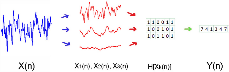
After calculating all the binary frequencies of interest, they were transformed into a single signal. This new signal was a sequence composed, at each time step, of integers, each of which symbolically represented the binary values at each scale as a single integer in base 2. Finally, for simplicity, these binary numbers were converted into base-10 integers (see Fig. 1 for a graphical description of the whole procedure). For example, if we obtained three binary sequences, and at time step t, the values of each were 1, 0, and 1, then we took the number 101 as a base 2 number, and transformed it to 5 in base 10. Note that in this case, 5 represents a state with specific information about the three rhythms obtained with each binary sequence.

Fig. 1

Graphical representation showing the steps to obtain the symbolic series Y(n) necessary for MIMR calculation. The first step is to obtain smoothed versions of the original signal and use them as thresholds to produce binary series H[Xk(n)]. Each column of this resulting binary matrix is considered a state of the system. In the example of the figure, the first column would be [1 1 1] which in a base 10 would be 7

From the integers in this symbolic series , we obtained the MIMR as the delayed mutual information

$$} = I\left( \right),$$

(1)

where the parameter τ can be estimated from the autocorrelation function of Y(n), and it was set to τ = 10. This measure provides the average number of predicted bits in Y(n) given the state Y(n − τ). It is a way to calculate to what extend a given state Y(n) of the signal would be predicted by the past state Y(n − τ). It evaluates, therefore, the linear and nonlinear temporal dependencies within a time series, and it has been used to quantify the linear and nonlinear statistical coupling between biomedical signals (Escudero et al. 2009). For a more detailed and formal description of the measure, see Ibáñez-Molina et al. (2020).

In the process of MIMR calculation for this study, we used different window sizes (WS: 14, 50, 100) to obtain the binary sequences necessary for Y(n). These window sizes were selected to approximately capture classical rhythms of θ (~ 5 Hz), α (~ 10 Hz), γ (~ 35 Hz), respectively. Given that the sampling rate of the EEG signal was 500 Hz, 500/14 would give an approximation of the 35 Hz wavelength. The same rationale could be applied to 50 and 100 window sizes.

Comparison metrics

With the aim to better interpret or validate the results obtained with MIMR, we included Sample Entropy and PAC analyses in theta–gamma and theta–alpha couplings.

Sample Entropy assesses the EEG signals from an informational perspective without considering explicit rhythmic interactions. Given that MIMR is also information-based, comparing it with Sample Entropy—a measure that captures statistical dependencies across all scales—provides insight into potential cross-frequency interactions at various scales.

PAC examines cross-frequency interactions through the lens of phase–amplitude interactions. A correspondence in the pattern of results between MIMR and PAC might indicate that MIMR captures similar physiological mechanisms as those involved in PAC. We conducted analyses on both control participants and patients across all electrode sites, applying the Modulation Index method as outlined by Tort et al. (2010). We generated three band-passed signal versions for each relevant frequency band using a zero-phase Finite Impulse Response (FIR) filter in EEGLAB: 33–37 Hz for the gamma band, 8–12 Hz for the alpha band, and 3–6 Hz for the theta band. The gamma band's amplitude and the phases of the alpha and theta bands were extracted using the Hilbert transform. Subsequently, to examine the influence of slower frequencies on the power of the gamma band, we computed the Modulation Index for both theta–gamma and alpha–gamma couplings.

Data analysis and results

To investigate the coupling between different frequency bands in patients and controls, we calculated MIMR for different combinations of window sizes (WS:14–50, WS:50–100, WS:14–100 and WS:14–50-100), assuming that we were mapping different combinations of frequencies (α-γ, θ-α, γ-θ, and α-θ-γ, respectively).

To examine the distribution of these differences between patients and controls in the cortical topology, we performed comparisons at the sensor level. Since, in most of the sensors the MIMR distribution was not normal, we conducted group comparisons using the Wilcoxon signed rank test. Due to the issue of multiple testing errors, p values of comparisons were corrected by calculating the false discovery rate using the Benjamini and Hochberg’s (1995) method. The analyses were performed with R version 4.0.3 (2020). All figures shown in this study were constructed with violin box-plots. These plots consisted of boxes delineating quartile information, with Q1 being the lower side, Q2 as the median represented as the central line, and Q3 the upper side. The length of the line represent the range of the data, and the colored curves illustrate the probability distributions.

WS:14–50 (alpha–gamma coupling)

First, we examined the coupling between a fast and a slow rhythm across the topological map in patients and healthy controls. The results of the comparisons between SCZ and Ctrl groups in each of the channels are represented graphically in Fig. 2. Quantitative information on the value of the U statistic and the p value associated can be found in Supplementary Material.

Fig. 2

Box-plot of MIMR obtained for 14–50 windows’ size (α − γ interaction) in each sensor for SCZ and Ctrl groups. Only significant differences are highlighted. For each test, a false discovery rate (FDR) correction was applied to correct for multiple comparisons and minimize false positives

As can be seen, there were hardly any differences between groups in MIMR, except in P8, where alpha–gamma coupling was significantly higher in controls than in patients.

WS: 50–100 (theta–alpha coupling)

Second, we analyzed the coupling between two slow frequencies, alpha and theta (see Fig. 3). Detailed results of these comparisons can be found in the Supplementary Material.

Fig. 3

Box-plot of MIMR obtained for 50–100 windows size (θ − α interaction) in each of the sensors for SCZ and Ctrl groups. Only significant differences are highlighted. For each test, a false discovery rate (FDR) correction was applied to correct for multiple comparisons and minimize false positives; * represents p < 0.05

As can be seen, we found significant differences between groups; theta–alpha coupling was greater in patients than in controls, in the right frontal–central region. Although not significant, this same trend was observed in many sensors, as well as the reversed effect at P8 that had been previously observed for alpha–gamma coupling.

WS: 14–100 (theta–gamma coupling)

Third, we compared the coupling between two extreme frequencies, one slow (theta) and one fast (gamma). The results are summarized graphically in Fig. 4 (for more detailed information see Supplementary Material).

Fig. 4

Box-plot of MIMR obtained for 14–100 windows size (θ − γ interaction) in each of the sensors for SCZ and Ctrl groups. Only significant differences are highlighted. For each test, a false discovery rate (FDR) correction was applied to correct for multiple comparisons and minimize false positives; * represents p < 0.05, ** represents p < 0.01

As can be seen in Fig. 4, the differences now appear bilateralized and with a frontal–central location. In addition, it is worth mentioning the high values but with reduced variability of MIMR in patients in the prefrontal region.

WS:14–50-100 (theta–alpha–gamma coupling)

So far, we have studied how the coupling between pairs of frequency bands differed between patients and controls along the scalp topology. In this section, we analyzed the coupling among three frequency bands (θ, α, and γ). Similar to the previous sections, additional detailed information can be found in the Supplementary Materials. A graphical summary of these comparisons is presented in Fig. 5.

Fig. 5

Box-plot of MIMR obtained for 14–50-100 windows size (θ–α–γ interaction) in each of the sensors for SCZ and Ctrl groups. Only significant differences are highlighted. For each test, a false discovery rate (FDR) correction was applied to correct for multiple comparisons and minimize false positives; * represents p < 0.05

In this case, we found significant differences between groups only in the right hemisphere.

Comparison metrics

To further explore the informational and coupling characteristics of the signals, we also conducted the Sample Entropy and theta–gamma and alpha–gamma PAC measures.

Sample entropy

As stated in the previous section, Sample Entropy was calculated to discriminate between patients and controls through scalp topology. None of the differences were significant. Detailed results of the comparisons can be found in Supplementary Material.

PAC measures

As indicated above, we calculated the Modulation Index as a PAC measure for theta–gamma and alpha–gamma. We applied the same statistical analysis to those in MIMR showing that there were no significant differences between control and patients at any electrode site (See Supplementary Material for details).