In the following sections, we describe the biomedical KG used in our research, the proposed framework for learning embeddings, and the evaluation protocols used to assess its performance.

The BioKG knowledge graph

BioKG is a Knowledge Graph built for the purpose of supporting relational learning in complex biological systems [38], with a focus on protein and molecules (interchangeably referred to as drugs). It was created in response to the problem of data integration and linking between various open biomedical knowledge bases, resulting in a compilation of curated data from 13 different biomedical databases, including DrugBank [12], UniProt [13], and MeSH [14].

The pipeline for creating BioKG employs a module to programmatically retrieve, clean and link the different entities and relations found in different databases, by reconciling their identifiers. This results in a biomedical KG containing over 2 million triples, where each entity has a uniform identifier linking it to publicly available databases. The coverage over multiple biomedical databases in BioKG presents a significant potential for training machine learning models on KGs with attribute data. Additionally, the availability of identifiers in BioKG facilitates the search for entity attributes of different modalities. These characteristics make BioKG an ideal choice for furthering research in the direction of machine learning on knowledge graphs with attribute data.

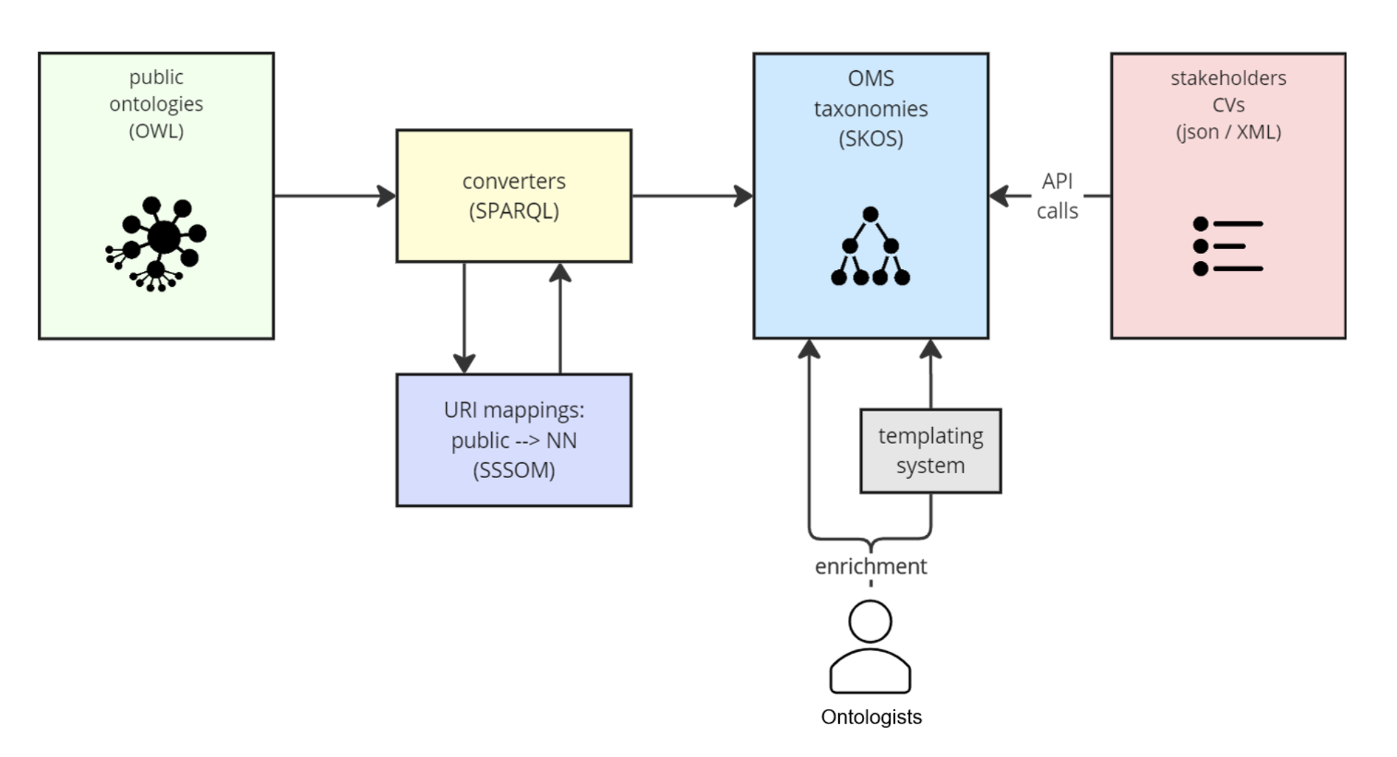
BioKG contains triples involving entities of 5 types: proteins, drugs, diseases, pathways, and gene disorders. We use the publicly available repositoryFootnote 1 to compile BioKG from the original sources, as available on May 2022. A visualization of the schema is shown in Fig. 2, and the statistics of the graph are listed in Table 1.

Fig. 2

Visualization of the entity types in the BioKG graph. Edges between nodes denote the existence of any relation type. Shaded nodes indicate entities for which we retrieve attribute data

Table 1 Statistics of the BioKG graph used in our work. The Attribute Coverage refers to the number of entities that have associated attribute data, which we retrieve for proteins, molecules, and diseases

Following our aim of learning embeddings that incorporate attribute data of different modalities, while taking into account entities with missing attribute data, we retrieve attributes for proteins, drugs, and diseases. To do so, we take advantage of the uniform entity identifiers present in BioKG, that allow us to query publicly available API endpoints. In particular, we retrieve amino acid sequences from UniprotFootnote 2, SMILES representations for drugs from DrugBankFootnote 3, and textual descriptions of diseases from MeSHFootnote 4. In a few cases where a textual MeSH scope note was unavailable for a disease, we use the text label for the disease as is, as this can contain useful information about the class, or anatomical categorization of a disease. We report the resulting coverage of attribute data for the entity types of our interest in Table 1. The result is a KG containing attribute data of three modalities for approximately 68% of the entities, while for the rest of the entities attribute data is missing, which are the desired characteristics of the KG for our research objective.

Biomedical benchmarks

One aspect that separates BioKG from other related efforts [7], is the inclusion of benchmark datasets around domain-specific tasks such as Drug-Protein Interaction and Drug-Drug Interaction prediction. This is crucial, as it allows for experimentation and comparison to standard benchmark datasets and approaches. The benchmarks consist of pairs of entities for which a particular relationship holds, such as an interaction between drugs. We use them for comparing the predictive performance of KG embeddings obtained when using the graph structure alone, and when incorporating attribute data. In total, five benchmarks are provided with BioKG, all considering different drug-drug and drug-protein interactions.

We focus on the DPI-FDA benchmark, which consists of drug target protein interactions of FDA approved drugs compiled from KEGG and DrugBank databases. It is comprised of 18,928 drug-protein interactions of 2,277 drugs and 22,654 proteins. This benchmark is an extension of the DrugBank_FDA [53] and Yamanishi09 [54] datasets which have 9,881 and 5,127 DPIs respectively. We refer to it as the DPI benchmark.

Data partitioning

In order to train and evaluate different KG embedding methods, we need to specify sets of triples for training, validation, and testing. Considering that the original BioKG dataset does not provide predefined splits, we generate our own. Since we aim to train multiple embedding methods on BioKG, and evaluate their performance over the benchmarks, we must guarantee that the KG and the benchmarks are decoupled, so that there is no data leakage from the benchmarks into the set of KG triples used for training.

Our strategy for partitioning the data is as follows:

1.

We merge the five benchmarks provided in BioKG into a single collection of entity pairs.

2.

For every pair of entities (x, y) in the collection, we remove all triples from BioKG in which x and y appear together, regardless of which one is at the head or tail of the triple.

3.

Removing triples from BioKG in step 2 might lead to the removal of an entity entirely from the graph.

4.

We split the resulting triples in BioKG into training, validation, and test sets, ensuring that all entities occur at least once in the training set of triples.

The last two steps are a requirement for lookup table embeddings. These methods require that all entities are observed in the training set of triples, so that we can obtain embeddings for evaluating i) link prediction performance on the validation and test triples, and ii) prediction accuracy on the DPI benchmark.

The proportions used for selecting training, validation, and test triples are 0.8, 0.1, and 0.1, respectively. We present statistics of the generated splits in Table 2. In the DPI benchmark, we end up with 18,678 pairs that we used to train classifiers and evaluate them via cross-validation.

To further research in this area, we make all the data we collected publicly available, comprising the attribute data for proteins, molecules, and diseases, and the splits generated for training, validation, and testing of machine learning models trained on BioKGFootnote 5.

Table 2 Statistics of the BioKG splits of triples used for training, validation, and testing, after removing triples overlapping with the benchmarksBioBLP

We now detail our new method, BioBLP, proposed as a solution to the problem of learning embeddings of entities in a KG with attributes. We design it as a extension of BLP [23] to the biomedical domain that incorporates the three data modalities available to us in the BioKG graph. BLP is a method for embedding entities in KGs where all entities have an associated textual description. At its core lies an encoder of textual descriptions based on BERT, a language model pretrained on large amounts of text [35]. In this work, we propose a more general formulation that considers multiple modalities as well as missing attribute data. By supporting KGs that contain entities with and without attributes, we can exploit the full extent of the information contained in the graph, rather than limiting the data available for training to one of the two cases.

BioBLP is a model for learning embeddings of entities and relations in a KG with attribute data of different modalities. It is comprised by four components: a set of attribute encoders, lookup table embeddings for entities with missing attributes and for relation types, a scoring function, and a loss function.

Attribute encoders Let \(G = (V, R, E, D, d)\) be a KG with attribute data. BioBLP contains a set of k modality specific encoders \(\lbrace e_1, \ldots , e_k\rbrace\). Each of the \(e_i\) are functions of the attributes of an entity that output a fixed-length embedding. If we denote as \(D_i\subset D\) the subset of attribute data of modality i (e.g. the subset of protein sequences), then formally each encoder is a mapping \(e_i: D_i\rightarrow \mathcal \), where \(\mathcal \) is the embedding space shared by all entities. We design the encoders as neural networks with learnable parameters, whose architecture is tailored to the input modality.

Lookup table embeddings For entities that are missing attribute data, we employ a lookup table of embeddings. For each entity in V with missing attributes, we assign it an initial embedding by randomly sampling a vector from \(\mathcal \). We follow the same procedure for all relations in R. These embeddings are then optimized, together with the parameters of the attribute encoders in F. In practical terms, this means that when attributes are not available at all, BioBLP reduces to lookup table embedding methods such as TransE [18]. We implement the lookup table embeddings via matrices \(\textbf_e\) and \(\textbf_r\) for entities and relations, respectively, with each of the rows containing a vector in \(\mathcal \). The embedding function of an entity without attributes is an additional encoder \(e_0\) such that \(e_0(h)\) returns the row corresponding to entity h in \(\textbf_e\). Similarly for relations, we define its embedding via a function \(e_r\) the retrieves the embedding of a relation from the rows of \(\textbf_r\).

Scoring function Once the attribute encoders and the lookup table embeddings have been defined, for a given triple (h, r, t) we can obtain the corresponding embeddings \(\textbf, \textbf, \textbf\in \mathcal \). These can be passed to any scoring function for triples \(f: \mathcal ^3\rightarrow \mathbb \), such as the TransE scoring function defined in Eq. 1. The scoring function also determines the type of embedding space \(\mathcal \). For TransE, this corresponds to the space of real vectors \(\mathbb ^n\) while for ComplEx and RotatE it is the space of complex vectors \(\mathbb ^n\).

Loss function The loss function is designed so that it can be minimized by assigning high scores to observed triples, and low scores to corrupted triples [51]. Corrupted triples are commonly obtained by replacing the head or tail entities in a triple (h, r, t) by an entity sampled at random from the KG. For such a triple, the loss function can thus be defined as a function \(\mathcal (f(\textbf, \textbf, \textbf), f(\tilde}, \textbf, \tilde}))\). An example is the margin ranking loss function:

$$\begin \mathcal (f(\textbf, \textbf, \textbf), f(\tilde}, \textbf, \tilde})) = \max (0, f(\tilde}, \textbf, \tilde})- f(\textbf, \textbf, \textbf) + m), \end$$

(2)

which forces the score of observed triples to be higher than for corrupted triples by a margin of m or more.

We optimize the parameters of the attribute encoders and the lookup table embeddings via gradient descent on the loss function. If we denote by \(\varvec\) the collection of parameters in the entity encoders plus the lookup table embeddings, the training update rule during for a specific triple is the following:

$$\begin \varvec^ = \varvec^ - \alpha \nabla _\theta \mathcal (f(\textbf, \textbf, \textbf), f(\tilde}, \textbf, \tilde})), \end$$

(3)

where t is a training step, \(\nabla _\theta\) is the gradient with respect to \(\varvec\) and \(\alpha\) is the learning rate. We outline the algorithm for training BioBLP in Algorithm 1.

Algorithm 1 BioBLP: Learning embeddings in a KG with entity attributes

Implementing BioBLP

The modular formulation of BioBLP is general enough to enable experiments with different choices for each of the modules, and presents an opportunity for incorporating domain knowledge into the design of different attribute encoders. In this section we describe the particular choices that we make for training BioBLP with the BioKG graph.

Considering that we retrieve attribute data for proteins, drugs, and diseases in BioKG, we define encoders for these three types. Recent works have demonstrated the effect of using pretrained embeddings in link prediction models that use textual descriptions [23, 32, 33]. Pretraining is done on a task for which a large dataset is available, such as masked language modeling [35]. Intuitively, the use of large pretrained models provides a better starting point for training, compared to randomly initializing an encoder and training for link prediction. In the context of the biomedical domain, we explore this strategy by considering three pretrained models as attribute encoders: ProtTrans [55], MolTrans [56], and BioBERT [57].

Protein encoder ProtTrans is a model for encoding amino acid sequences of proteins, where each of the input tokens is an amino acid [55]. The output is a matrix of “contextualized” amino acid embeddings of size \(n_e\times l\), where l is the length of the sequence and \(n_e\) the dimension of the ProtTrans embeddings. Encoding proteins with ProtTrans in BioKG is challenging: we found that some sequences can have lengths up to 35,213, which greatly increases memory requirements. To reduce memory usage during training, we choose not to optimize the parameters of the ProtTrans encoder. Given the output matrix of amino acid embeddings, we obtain a single protein embedding by taking the average over the sequence, and then linearly projecting the result to the embedding space of dimension n via a matrix of size \(n\times n_l\) with learned parameters. The reason for averaging the embeddings is that due to computation constraints, it is not feasible to fine-tune the ProtTrans encoder. If fine-tuning the encoder were feasible, it would be possible to use the embedding of a special marker at the beginning of the sequence. We thus use the average as an aggregated representation.

Molecule encoder MolTrans is a model initially trained to learn representations of molecules, by translating them from their SMILES representation to their IUPAC name [56]. We use it to obtain embeddings for molecules in BioKG for which we have a SMILES representation. The output of MolTrans is a matrix of embeddings of size \(n_e\times l\), where l is the length of the SMILES string and \(n_e\) is the size of the MolTrans embeddings. Similar to the case of the protein encoder, we do not optimize the parameters of MolTrans due to memory constraints. Instead, we apply a layer of self-attention [58] and select the output embedding at the first position, which corresponds to a special marker for the beginning of the sequence. This embedding is then linearly projected to an embedding of size n, and the result is used as the embedding of the molecule. In the case of the molecule encoder, the learnable parameters are the weights in the self-attention layer, and the linear projection matrix.

Disease encoder We rely on BioBERT [57] to encode textual descriptions of entities. BioBERT is a language model trained to predict words that have been removed from some input text, which is also known as the masked language modeling task [35]. In contrast to models like BERT [35] that have been trained over diverse sources from the internet, BioBERT has been pretrained with scientific articles obtained from PubMed and PMC. Given an input textual description, we select the output embedding of the special marker at the start of the description, and then project it to an embedding of size n. As opposed to the protein and molecule encoders, we optimize all the layers in the BioBERT encoder as well as the projection layer. We can afford this by limiting the length of the descriptions to a maximum of 64 tokens, which helps to curb the memory requirements during training. Previous work has shown that further increasing the length of text encoders for embedding entities in KGs brings dimishing returns [23].

Choice of pretrained encoder models. An important tradeoff between computational complexity and accuracy arises when selecting encoders. While state-of-the-art methods can provide better representations [59], we prioritized publicly available encoders that would fit within our computation budget.

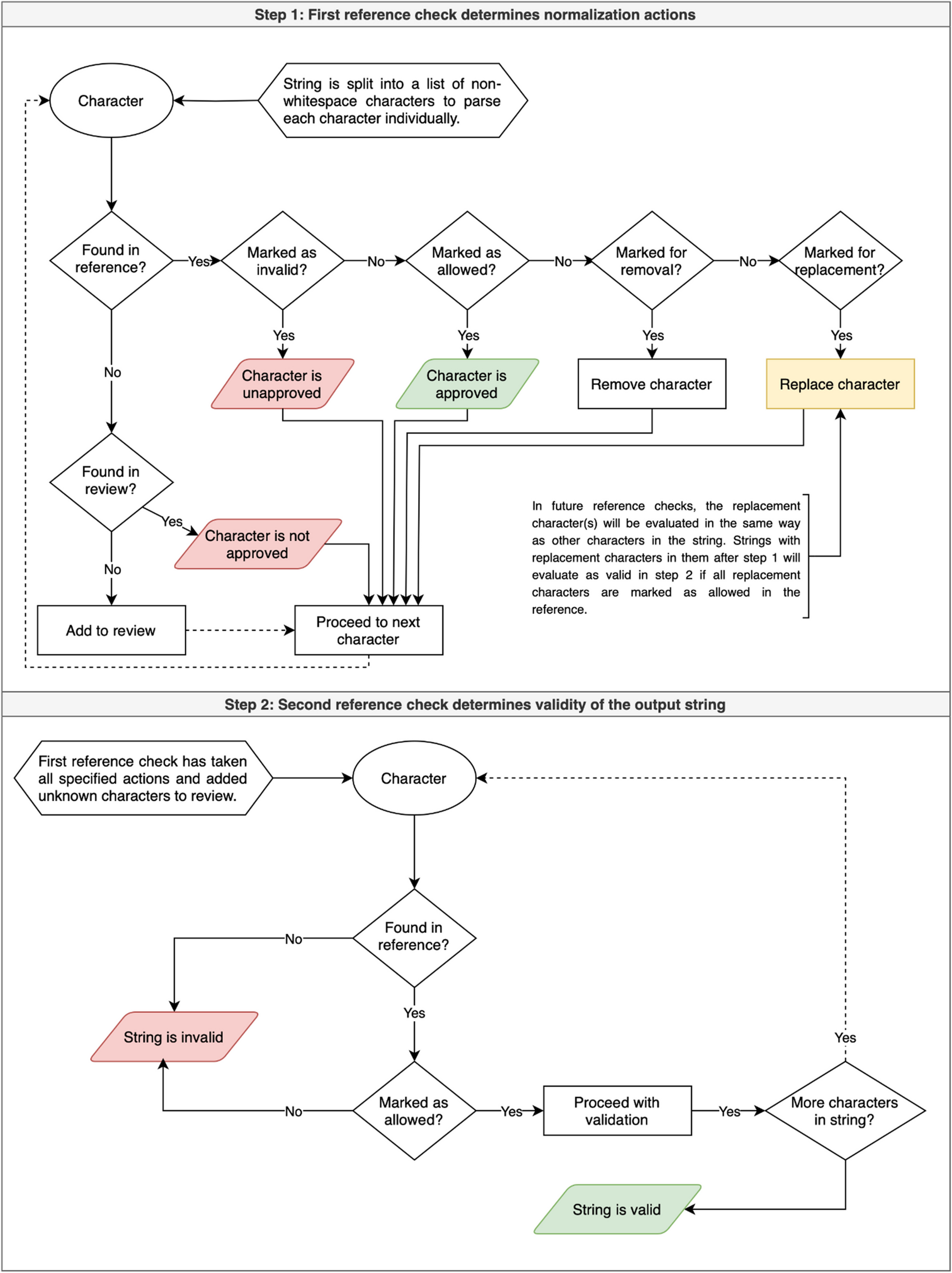
In summary, we provide an implementation of BioBLP for the BioKG graph that uses encoders of amino acid sequences for proteins, SMILES representations for molecules, and textual descriptions of diseases. Following the BioBLP framework, other entity types like pathways and gene disorders are embedded using lookup table embeddings. We illustrate the architecture in Fig. 3.

Previous research has shown that in spite of continuous developments in the area of KG embeddings, the choice of scoring function is a matter of experimentation and the results are highly data-dependent [23, 50, 51]. For these reasons, we experiment with three scoring functions: TransE [18], ComplEx [19], and RotatE [20]. For the loss functions, we consider the margin ranking loss, the binary cross-entropy loss, and the cross-entropy loss [51]. Our implementation uses the PyKEEN library [60] and is publicly availableFootnote 6.

Fig. 3

The architecture of BioBLP for the BioKG graph. On the left we illustrate the graph with the three entity types that have attribute data: proteins (P), molecules (M, representing drugs), and diseases (D). We omit entity types without attributes for clarity. For the three types, we retrieve relevant attribute data, which are the inputs to encoders for each modality. The output of the encoders is a vector representation of the entities

Efficient model pretraining

Training KG embedding methods that use encoders of attribute data has been shown to significantly increase the required computational resources for training [23, 32, 33]. Furthermore, BioBLP consists of a set of attribute encoders, together with lookup table embeddings for entities with missing attributes. Training such a model from scratch requires all the encoders to adapt together for the link prediction objective. If lookup table embeddings are initialized randomly as is customary, attribute encoders will adjust to their random-level performance, greatly slowing down the rate of learning. We thus propose the following strategy to overcome this problem:

1.

Train a BioBLP model with lookup table embeddings for all the entities in the graph.

2.

Train a BioBLP model with encoders for entities with attribute data, and for entities without such data, initialize their lookup table embeddings from the model trained in step 1.

Step 1 is much cheaper to run since it does not make use of any attribute encoders. This speeds up training, and facilitates hyperparameter optimization. In step 2, the encoders no longer have to adapt to randomly initialized lookup table embeddings, but to pretrained embeddings that already contain useful information about the structure of the graph, which reduces the number of training steps required.

Answering RQ1 Given the question, “How can we incorporate multimodal attribute data into KGE models under a common learning framework?”, we find that

A survey of the literature shows that existing methods ignore attribute data, or assume a uniform modality (such as text) for all entities.

We design BioBLP as a method that enables the study of the effect of incorporating multimodal data into knowledge graph embedding, under a common learning framework where all encoders are optimized jointly.

We propose a strategy for efficient model pretraining that improves the practical application of BioBLP.

Evaluation

In our experiments, we aim to answer research questions RQ2 and RQ3, related to how the different attribute encoders in BioBLP compare with traditional KG embedding methods that rely on the structure of the graph only.

We focus on two tasks to answer this question: link prediction, and the DPI benchmark present in BioKG.

Link prediction

The link prediction evaluation is standard in the literature of KG embeddings [50, 51]. Once the model is trained, the evaluation is carried out over a held-out test set of triples that is disjoint from the set of triples used during training.

For a triple (h, r, t) in the test set, a list of scores for tail prediction is obtained by fixing h and r and computing the scoring function \(f(\textbf, \textbf, \textbf)\), for all possible entity embeddings \(\textbf\). The list of scores is sorted from high to low, and the rank of the score for the true tail entity t is determined. We repeat this for all triples in the test set, collecting a list of ranks for tail prediction. For head prediction, the process is similar, but instead we fix r and t and collect the ranks of the true head entity h given scores for the head position. We collect the ranks for head and tail prediction in a list \((p_1, \ldots , p_m)\). From this list we compute the Mean Reciprocal Rank, defined as

$$\begin \text = \frac\sum \limits _^m \frac, \end$$

(4)

and Hits at k, defined as

$$\begin \text = \frac \sum \limits _^m \mathbbm [p_i \le k], \end$$

(5)

where \(\mathbbm [\cdot ]\) is an indicator function equal to 1 if the argument is true and zero otherwise.

It is important to note that by averaging over the set of evaluation triples, these metrics are more influenced by high-degree nodes, simply because they have more incident edges. This means that it is possible that a model can score highly in the link prediction task by correctly predicting edges for a small number of entities that account for a significant number of the triples in the graph [61].

We use the MRR and H@k metrics to report the performance of the embeddings obtained with BioBLP. As baselines that do not incorporate attribute data, we consider TransE, ComplEx, and RotatE. For a direct comparison, we experiment with variants of BioBLP that use the same scoring functions as in these baselines. This allows us to determine when improvements are due to the choice of scoring function, rather than a result of incorporating attribute data.

Hyperparameter study Previous research has shown that KG embedding models and the optimization algorithms used to train them can be sensitive to particular choices of hyperparamenters [50], including in the biomedical domain [52]. Hence, a key step in determining the performance of our baselines against models that incorporate attributes is an exhaustive optimization of their hyperparameters. For each of the three baselines we consider, we carry out a hyperparameter study with the aim of optimizing their performance before comparing them with BioBLP. We focus on four hyperparameters as listed in Table 3, where we also describe the intervals and values we considered. For each baseline, we used Bayesian optimization to search for hyperparameters, running a maximum of 5 trials in parallel. We ran a total of 90 different hyperparameter configurations with TransE, 180 with ComplEx, and 180 with RotatE. For TransE we only consider the margin ranking loss function, while for ComplEx and TransE we experiment with the binary cross-entropy and cross-entropy, which leads to twice the number of experiments.

Table 3 Intervals and values used in the hyperparameter study we carried out to optimize the TransE, ComplEx, and RotatE baselinesBenchmarks

We evaluate the utility of entity embeddings by testing their performance as input features for classifiers trained on related biomedical tasks. We focus on the DPI benchmark obtained from BioKG. As it is common in literature, we interpret this task as binary classification [62,63,64]. We use the pairs in the benchmarks as positive instances to train the classifiers. A common issue in modelling efforts in biomedical domain is the lack of true negative samples in public benchmark datasets. Therefore, we sample negatives from the combinatorial space assuming a pair that is unobserved in the dataset is a candidate negative sample [39, 62,63,64]. Furthermore, we filter out any triples appearing in BioKG from the list of candidate negatives. We use a ratio of positive to negatives of 1:10.

For a given pair of entities, we concatenate their embeddings into a single vector that is used as input to a classifier. We evaluate a number of baselines for computing embeddings, including random embeddings, entity embeddings that do not rely on the graph, and KG embeddings. We compare these to embeddings obtained with BioBLP. In particular, we use the following embeddings:

Random. Every entity is assigned a randomly generated feature vector from a normal distribution. We use this method to determine a lower bound of chance performance. Each entity is assigned an 128-dimensional embedding.

Structural. Drug entities are represented by their MolTrans embeddings of 512 dimensions, and proteins are represented by their ProtTrans embedding, averaged across tokens resulting in a 1024-dimensional vector.

KG. Entities are represented by TransE, ComplEx, and RotatE embeddings trained on BioKG. The entity embeddings from these models all have 512 dimensions.

BioBLP. Entities are represented from the attribute encoders in BioBLP models trained using the RotatE scoring function, on the BioKG graph. The entity embeddings from the BioBLP-D, BioBLP-M and BioBLP-P models have 512 dimensions.

When using Structural Embedding, it may occur that a particular entity does not have a corresponding feature, for example, because we are missing the chemical structure embeddings for a set of molecules (as detailed in Table 1) because these are biologic therapies and do not have a SMILES property. In these cases, we impute the missing embeddin