
Remember me


We analyzed the public-access dataset from the NIAAA-supported National Epidemiologic Survey on Alcohol and Related Conditions (NESARC), Wave I study [12]. The NESARC was a nationally representative study of adults 18 years or older (N = 43,093) who were interviewed face-to-face using the Alcohol Use Disorder and Associated Disabilities Interview Schedule-DSM-IV (AUDADIS-IV). The NESARC sampled sociodemographic subgroups to ensure that the sample sufficiently represented the US population (e.g., Hispanic, Non-Hispanic Black, and young adults) with a response rate of 81%. From the total number of respondents, 7,839 met criteria for an MDE in their lifetimes. Participants were excluded from our analyses if they A) met criteria for mania or hypomania (n = 725), or B) their worst episode experienced was deemed illness or substance-induced (n = 715). After exclusion criteria were applied, 6,448 possible MDE cases (82.3%) remained. From this pool, participants that had missing depression symptom data were listwise deleted, leading to a final count of n = 5,749 participants (73.3%). In the NESARC, participants reported symptoms on their worst depressive episode within their lifetime. Thus symptom data were drawn retrospectively from episodes over the course of the participant’s lifetime.
STAR*DWe also re-analyzed the Sequenced Treatment Alternatives to Relieve Depression (STAR*D; [13]). The STAR*D is a multi-site sequentially randomized clinical trial of 4,041 outpatients who were diagnosed with major depressive disorder (MDD). Inclusion criteria included being between the ages of 18 and 75 and a diagnosis of DSM-IV unipolar and non-psychotic MDD. Exclusion criteria included a history of mania or hypomania, schizophrenia, schizoaffective disorder or psychosis, or current anorexia, bulimia, or obsessive-compulsive disorder (OCD) as assessed by the Psychiatric Diagnostic Screening Questionnaire (PDSQ) via clinical interview [14]. Depressive symptoms, including melancholic and atypical symptoms, were screened using the Inventory of Depressive Symptomatology (IDS-SR). For more information regarding the study design, please refer to the following studies [4, 13]. The original sample had data available for 4,041 patients. Of these patients, 3744 (92.7%) provided baseline data during the first measurement point of the first treatment stage. We screened out patients who did not have full symptom-level IDS data, leading to 3,717 patients (91.9%). Inclusion criteria in the original trial required patients to meet the criteria for non-psychotic MDD based on a DSM-IV checklist. To ensure consistency, patients were screened for meeting an MDE based on the IDS itself, leading to n = 2,498 remaining patients (61.8%). Patients were queried on specific symptoms based on their current depressive episode. Thus, we derived diagnostic combinations from the STAR*D patients’ current depressive episode. See Lorenzo-Luaces et al. (2021; [8]) for a description of how the STAR*D symptoms were parsed.
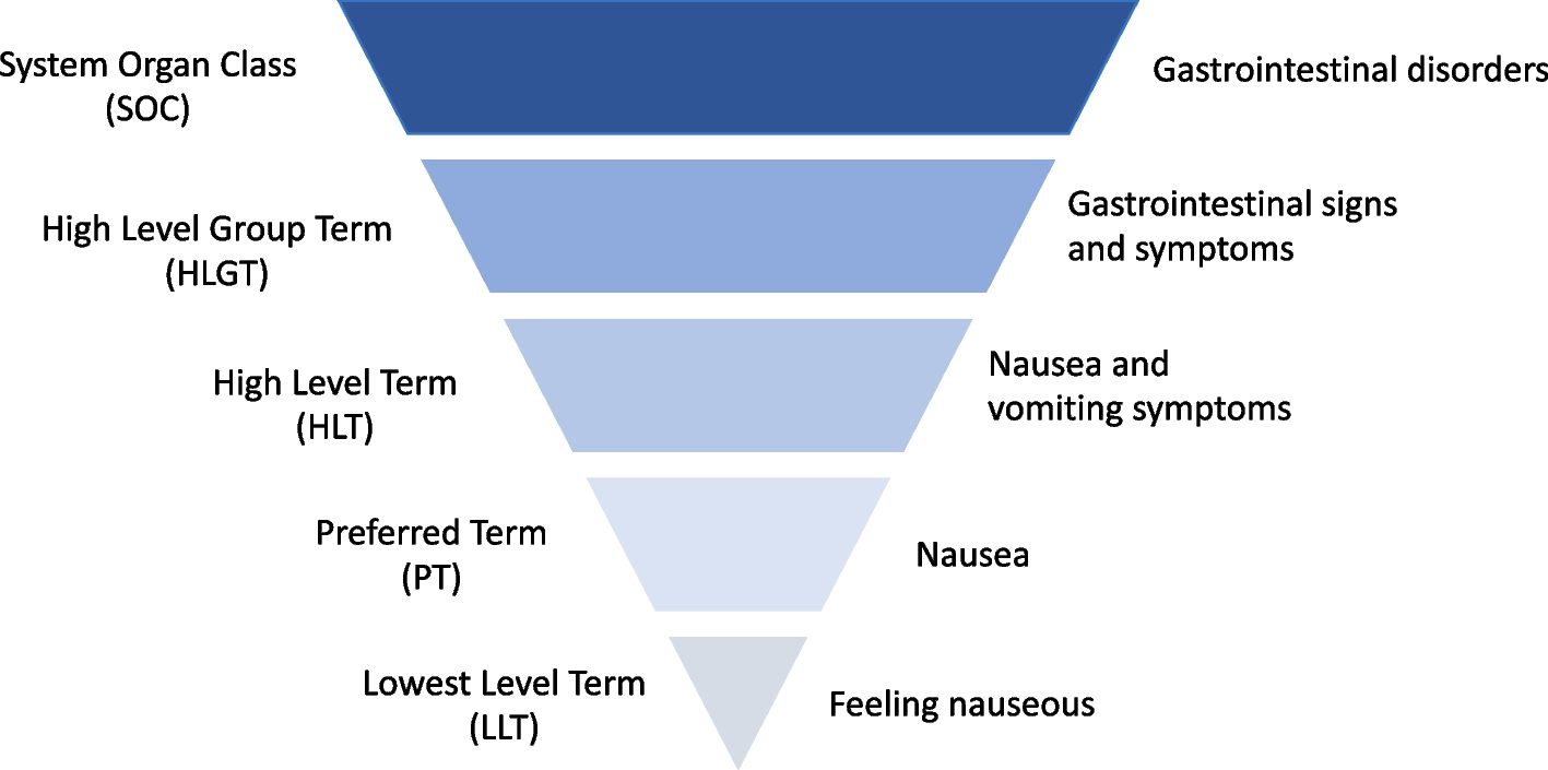
Outcomes Alcohol Use Disorder and Associated Disabilities Interview Schedule (AUDADIS-IV)In NESARC, the AUDADIS-IV [15] measures 19 symptoms of depression that are rated as either ‘present’ or ‘absent’ and coded as “1” or “2”, respectively. The AUDADIS-IV covers DSM-IV criteria symptoms in a disaggregated form. For example, it queries both psychomotor agitation and psychomotor retardation, whereas the DSM-IV codes psychomotor disturbances as a single symptom. In the end, we evaluated similarity across 16 symptoms. Below, we describe our decision-making process regarding symptom inclusion in the NESARC dataset.
Appetite or weight disturbancesThe AUDADIS-IV contains four questions querying appetite or weight disturbances: 1) reduced appetite, 2) reduced weight, 3) increased appetite, and 4) increased weight. To prevent over-estimating the degree of heterogeneity in the data from overlapping symptoms, we combined the responses to the appetite and weight questions, thus creating two variables: 1) decreased appetite or weight and 2) increased appetite or weight. For decreased appetite/weight, we considered the person to have the symptom whether they reported decreased appetite, decreased weight, or both. Similarly, for increased appetite or weight, we considered the person to have the symptom whether they reported increased appetite, increased weight, or both.
Suicidal ideationThe AUDADIS-IV contains four questions pertaining to suicide: 1) death ideation (i.e., thoughts of death), 2) desire to die, 3) suicidal ideation (i.e., thoughts about killing oneself), and 4) attempted suicide. We distinguished suicidal attempts from thoughts by combining the responses to the first three questions (i.e., death ideation, desire to die, and suicidal ideation) into a symptom indicating the presence of suicidal thoughts. A person was considered to have suicidal thoughts if they expressed death ideation, desire to die, suicidal ideation, or some combination of these symptoms.
Restlessness and psychomotor agitationThe AUDADIS-IV queries an uncomfortable feeling of restlessness as well as symptoms of fidgeting and pacing as proxies for psychomotor agitation. We removed the ’feelings of restlessness’ symptom when performing the analyses, as subjective feelings of restlessness do not count towards the presence of psychomotor agitation per the DSM-5 (American Psychiatric Association, 2013).
Melancholic and atypical specifiersThe AUDADIS-IV does not query all the symptoms of melancholic and atypical depression. We categorized melancholic depression as having three symptoms from a list that included: anhedonia, psychomotor retardation/agitation, guilt, early morning awakenings, or significant weight loss. Comporting to previous NESARC analyses [16], the atypical subgroup consisted of respondents who met criteria for both hypersomnia and hyperphagia. The hierarchical rule of specifiers was also applied: Participants meeting criteria for a melancholic specifier could not then meet criteria for an atypical specifier (see appendix for a list of queried symptoms and criteria rules). The STAR*D dataset used the IDS to query for all depressive symptoms, including those for the melancholic and atypical specifiers. Thus, we adhered to the DSM-5’s criteria for melancholic and atypical specifiers in the STAR*D analyses.
Analytic strategySimilar to previous analyses [8], we divided the NESARC and STAR*D datasets into subgroups corresponding to the presence of melancholic and atypical specifier subgroups, as shown in Fig. 1. Because we respected the hierarchical rule from DSM-5, all participants were screened for the presence of melancholia first, creating melancholic and non-melancholic subgroups. Then, all participants in the “non-melancholic” group were grouped into atypical vs. non-atypical subgroups.
Fig. 1
Melancholic and Atypical subgroups of patients derived from the IDS on the STAR*D (A) and AUDADIS-IV on the NESARC (B) datasets
All data were analyzed using the R programming language. All code is available at: https://osf.io/vh5qg/. Two functions calculating distance in N-dimensional space, known as the Hamming and Manhattan distances, were used [17, 18]. The Hamming formula is a way to measure distance in an N-dimensional space given two binary data strings (i.e., data containing only 0s and 1s). Equation 1a represents the formula for the Hamming distance (DH) for a dyad composed of person x and person y. DH is calculated by summing the differences of two vectors in a vector space of symptoms represented by variable k, here representing the maximum number of possible symptoms. The term xi, represents symptom i within vector-space k of patient x, and yi represents the same symptom i of patient y. For every specific symptom that is not shared between any two diagnostic combinations, the Hamming distance between the diagnostic combinations will increase by 1. Since the symptoms in NESARC were assessed as a binary, we used Hamming distances to calculate distances between individuals in their symptom endorsement.
Equation 1: Hamming Distance Function
$$\begin D_H = \sum \limits _^ |x_i - y_i| \end$$
(1a)
$$\begin R_H = \frac \end$$
(1b)
Similar to the Hamming distance, the Manhattan distance quantifies the distance between two symptom vectors in an N-dimensional vector space k, which again refers to the total number of symptoms, as shown in Eq. 2a. The Manhattan distance for person x and person y, represented by DM, is calculated by summing the differences between two symptom profiles in a vector space of symptoms k, where xi represents symptom i of patient x, and yi represents the same symptom i of patient y. The Manhattan distance allows us to quantify distance in kind (i.e., symptom present vs. absent) as well as intensity (i.e., mild vs. severe presentations of the same symptom: see equation 2). A higher Manhattan distance between the diagnostic combinations of two individuals indicates a greater dissimilarity between them in the severity and kinds of symptoms. The Manhattan distance is not equivalent to a total sum score. Two combinations of symptoms can have equal total sum scores that arise from different symptom endorsements and would result in different Manhattan distances (see Appendix). Given that symptoms on the IDS were assessed on a polytomous 4-point scale, Manhattan distances were calculated for the STAR*D dataset.
Equation 2: Manhattan Distance Function
$$\begin D_M = \sum \limits _^ |x_i - y_i| \end$$
(2a)
$$\begin R_M = \frac \end$$
(2b)
To simplify interpretation, all distance measures were standardized by dividing distance values by the length of the total possible symptom space. Equation 1b represents the standardized Hamming ratio score RH, where DH is the calculated hamming distance, and the denominator is represented by the total number of symptoms queried or the maximum length of vector space k. Similarly, Eq. 2b displays the Manhattan ratio RM, which is calculated by dividing the total Manhattan distance DM by the maximum length of vector space k. Because the Manhattan distance takes into account symptom severity we also divided by the scalar v, representing the maximum possible severity score. It should be noted that the STAR*D and NESARC datasets queried a different number of symptoms, thus the number of symptoms in vector space k differed between the two datasets.
Several separate sets of analyses were conducted. The first set of analyses used the NESARC dataset to calculate Hamming distances for each subgroup (i.e., melancholic vs. non-melancholic, and atypical vs. non-atypical) for the depressive symptoms present in the dataset for both within and between subgroups. We also calculated standardized Hamming and Manhattan distances in the STAR*D dataset. Given that the IDS assesses symptoms of depression as well as the symptoms of the specifiers, we conducted two additional sets of analyses. One that had all the symptoms of depression plus the specifiers, and another that only had the core DSM-5 symptoms of depression.
For each analysis, we calculated the within and between-group standardized distance. Within-subgroup calculations consisted of comparing each person in each diagnostic subgroup to each other person in that subgroup. For example, when evaluating Subgroup “A” (e.g., melancholic depression in STAR*D), the diagnostic combination of person Ca1 was compared to the diagnostic combination of persons Ca2, Ca3, ... Can. Similarly, diagnostic combination Ca2 was compared to Ca3, Ca4, ... Can. A distance metric was calculated between every other person only once within that subgroup and stored into a vector containing all calculated distances. Between-subgroup distance calculations compared each person’s symptom combination in a subgroup to each participant not meeting subgroup criteria (e.g., non-atypical profiles with atypical profiles). A standardized distance score was computed for each pairing and then stored into a vector containing all distances.
Due to the size of the datasets, the within-group and between-group vectors of distances comprised millions of data points. Thus, we illustrate all analyses using box plots to avoid data overcrowding. Three example boxplots are provided in Fig. 2, demonstrating how within-subgroup and between-subgroup analyses may be interpreted. Panel A shows an ideal case of subgroup coherence and differentiation (i.e., where subgroups show the maximal distance between diagnostic combinations). Subgroup 1 and Subgroup 2 are approaching pure coherence, as the distance ratios are 0; simultaneously, the two subgroups appear to be distinct, having high differentiation as the between-subgroup ratio approaches 1.
In contrast, Fig. 2 Panel B displays a case of complete heterogeneity. Both within- and between-subgroup analyses exhibit nearly identical distance ratios. The between-subgroup ratio indicates that the subgroups are low in differentiation (i.e., the diagnostic profiles in both subgroups are similar to each other), whereas the identical within-subgroup ratios indicate both subgroups are similarly heterogeneous.
Finally, in Fig. 2 Panel C, we show a “mixed” scenario where the specifier groups could capture a homogeneous subgroup of patients (with distance scores of 0), but the non-specifier group is still heterogeneous (e.g., with distance scores around 0.5). In such a scenario, we would still see large between-group distances (0.75) and this would be an indication of the specifier reducing diagnostic heterogeneity. Indeed, this example would be more likely the case than Fig. 2 Panel A, if these specifiers were creating more coherent subgroups.
To rule out the possibility that the differences observed between specifier groups could be accounted for by chance, we conducted a series of permutation tests as in our previous study [8] to test whether the between-group differences were above and beyond what would be expected by chance. We conducted the permutation tests by randomly shuffling the specifier and non-specifier labels, obtaining a random dyad, and then obtaining distance scores for that dyad. We repeated this process 100 times for each between-group distance we present (i.e., for each specifier, for each dataset, for each set of symptoms). The p-values represent the probability that one would obtain a between-group distance as or more extreme than the one we observed by random chance.
Fig. 2
Illustration of distance ratios indicating ideal inner-group coherence and between-group differentiation between subgroup profiles, where subgrouping would be effective (A) heterogenous subgroup profiles generated using random data where subgrouping would be ineffective (B), and a mixed scenario where a homogeneous subgroup exists and subgrouping would be effective (C)
Comments (0)