Patients being investigated for suspected or confirmed cancer often undergo multiple imaging tests to ascertain the initial TNM stage before formulating the final treatment strategy. The multicenter prospective NIHR Streamline studies compared the diagnostic accuracy of whole-body magnetic resonance imaging (WB-MRI) with standard staging pathways (CT ± regional MRI [rectum, liver, brain] ± FDG PET/CT), for initial staging in patients with newly diagnosed non–small cell lung or colorectal cancer.1,2 The studies also evaluated the number of tests required and the time taken before reaching the final treatment plan. The Streamline studies found that WB-MRI is a viable alternative to standard pathways with similar accuracy but reduced staging time and cost.1,2 However, WB-MRI has not yet been widely translated into staging pathways in lung and colon cancer, although there is more widespread use for staging bone disease in myeloma and to some extent in prostate and breast cancer.3–5 One speculative reason for this could be due to a perceived need for specialist expertise in reading WB-MRI, as well as the time taken to report the scans, due to the challenges of integrating a large number of complex sequences available on WB-MRI.

Significant developments in machine learning (ML), especially deep learning (DL), have opened the possibility of automated segmentation and lesion detection on CT and MRI.6–11 However, ML techniques for cancer lesion detection on WB-MRI have not been widely researched.

The aim of this study was to develop and clinically test an algorithm for cancer lesion detection on WB-MRI scans in patients recruited to the Streamline studies with lung and colorectal cancer, using a human-in-the-loop approach. The intended use of the algorithm was a concurrent ML heat map on WB-MRI images at the time of interpretation, alerting radiologists to potential metastases, with the hypothesis that ML support would improve lesion detection and reduce read-times. Secondary objectives included evaluating reader performance for inexperienced WB-MRI readers and detection of the primary tumor with or without ML.

MATERIALS AND METHODS Study Design

This retrospective study obtained ethical approval (ICREC 15IC2647, ISRCTN 23068310). Patients gave written consent in Streamline studies (ISRCTN43958015 and ISRCTN50436483) for use of deidentified data for future research. TNM stages for each case were provided by the source study.

Scans were acquired at 16 recruitment sites between February 2013 and September 2016, using a minimum WB-MRI protocol.12 The Streamline consensus reference standard for sites of disease was used.1,2 In brief, this consisted of multidisciplinary consensus meetings, which retrospectively considered all imaging, treatment interventions, histopathology, and patient outcomes for at least 12 months after cancer diagnosis to ascertain the cancer stage and site of metastasis at diagnosis.

Cases were randomly allocated to model training and clinical testing (stratified by primary tumor type [lung or colon], presence of at least 1 metastatic lesion, and recruitment site), ensuring sufficient cases with and without metastases were allocated to the testing set to meet the power calculation, with all other cases allocated to training.

Data Preparation

All DICOM data received were initially included. Individual anatomical imaging stations of the 3 key sequences (defined as axial T2-weighted [T2WI], diffusion-weighted [DWI], or apparent diffusion coefficient [ADC] map) were stitched into a single DICOM stack and converted to NIfTI (https://nifti.nimh.nih.gov/).11,13 Cases were excluded due to absence of a key sequence or technical failure (NIfTI conversion or running the algorithm).

All visible disease sites (primary tumor and metastases) were segmented by trained radiologists using ITK-Snap, on T2WI and DWI NIfTI volumes based on the location, size, and number of lesions identified by the Streamline trials reference standard.14 Not all sites could be identified on the WB-MRI, as the source reference standard included metastases that subsequently became radiologically visible within 6 months, considering them likely present (although occult) at initial staging (see Supplemental Digital Content 1, https://links.lww.com/RLI/A825, which shows the visible sites for ground truth segmentation against the reference standard).

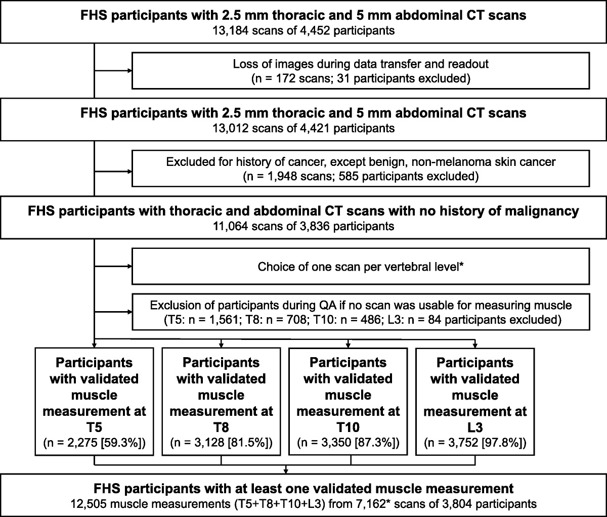
Data Availability

Among 486 patients in the Streamline studies, 438 WB-MRI scans were available for the study (270 colorectal and 168 lung cancer, 114 with metastases) (Fig. 1). The stages of disease are provided in Table 1.

FIGURE 1:

CONSORT diagram demonstrating distribution of cases to phase 2 training, with internal validation data set and phase 3 clinical test data set. C = colon cancer, L = Lung cancer.

TABLE 1 - Stage Distribution of the Cases Allocated to Radiology Reads (Test Set, n = 188) Number % Colon cancer stage n = 117  T1 7 6  T2 25 21  T3 69 59  T4 16 14  N0 55 47  N1 35 30  N2 27 23  M0 87 74  M1 30 26 Lung cancer stage n = 71  T1a 10 14  T1b 9 13  T2a 18 25  T2b 8 11  T3 14 20  T4 12 17  N0 42 59  N1 10 14  N2 13 18  N3 6 8  M0 51 72  M1 20 28

Among 245 scans allocated to training, there were 19 technical failures with 226 evaluable for training (n = 181) and internal validation (n = 45). Among 193 scans allocated to the test set, there were 5 technical failures (missing ADC n = 2, corrupted DWI n = 1, failure of NIFTI conversion and upload n = 2), leaving 188 evaluable scans (117 colon, 71 lung, 50 cases with metastases).

Machine Learning Model

We investigated several ML algorithms and different training strategies for the task of malignant lesion segmentation in multichannel WB-MRI. Details about the tested alternatives can be found in the Supplemental Digital Content 2, https://links.lww.com/RLI/A826. The final ML model was based on deep convolutional neural networks (CNNs), developed with a 2-stage strategy. We first leveraged an existing CNN algorithm for the segmentation of healthy organs, developed in a previous healthy volunteer study.11 Running this multiorgan CNN segmentation algorithm on all the training data provided automatic organ maps for all patient scans. This required an intermediate step of registering phase 2 data with a rigid registration algorithm to a template subject from the healthy volunteer data (Fig. 2). This was to compensate for the different fields of view of the healthy volunteer study and the current patient study. Although the healthy volunteer WB-MRI data covered the body from shoulders to knees, the patient study data included the head, which affects the performance of the organ segmentation algorithm. The registration was automatic and fast, and was only required in order to obtain the organ masks. The organ masks were then mapped back with the inverse transformation to the original patient training data. For the patient training data set, there was no reference segmentation of organs to compare with, so we assessed the quality of these segmentations visually, and they appeared to be sufficient for the second stage.

FIGURE 2:

Data generation process for the 2-stage model training approach. Panel A: A, An example of a T2WI WB-MRI scans from a participant in training set. B, After registration to a template scan from the healthy volunteer study. C, Output of the organ. Segmentation algorithm developed in healthy volunteer study. D, After mapping the organ segmentations back to the original scan from training data. E, Manual lesion segmentation overlaid on the T2WI scan. F, Merged organ segmentations and cancer lesion segmentation overlaid on the T2WI scan, which is used for training the final multiclass segmentation algorithm. Panel B: Cancer lesion detection training. A, Input T2WI scan (different patient to panel A). B, Diffusion-weighted scan. C, Manual lesion segmentation (based on reference standard) from T2WI image overlaid on diffusion scan. D, Postprocessed lesion probability map from the convolutional neural network (CNN) algorithm (deep medic). E, Postprocessed lesion probability map from the classification forest (CF) algorithm.

The automatically generated organ maps were then merged with the manually segmented primary and metastatic malignant lesions on T2WI and DWI training data (Fig. 2). This resulted in all scans allocated to training having multiclass segmentation maps where the organ labels were generated automatically using the previously developed CNN algorithm, although the cancer lesions were labeled manually. We then used the training set for training a CNN for joint organ and lesion segmentation, using the DeepMedic architecture.15 This CNN model was then capable of predicting jointly the organ labels and malignant lesions on new unseen test data. The generated probability heat maps for the lesion class were postprocessed by applying Gaussian smoothing with a kernel size of 5 mm, normalized to the range [0, 1], and thresholded to reduce false-positive predictions. Parameters for the postprocessing were selected based on visual assessment of the 45 internal validation cases. The final lesion probability heat maps were converted to DICOM and uploaded to PACS to enable overlay with the original WB-MRI scans. Each WB-MRI scan was copied (one with and one without ML heat map series) to allow masking.

Radiology Reads

Eighteen experienced readers were Streamline radiologists (n = 7) or those routinely reporting WB-MRI for tumor boards (n = 11). Seven inexperienced readers included consultants who do not read WB-MRI (n = 3) and board-certified senior radiology trainees (n = 4). All readers were trained to use the Biotronics3D reading platform, including optional superimposition of ML heat maps (see Supplemental Digital Content 3, https://links.lww.com/RLI/A827, which shows the reader training manual with appearance of the PACS reading setup with heat maps).

Cases in the test set (n = 188) were randomly allocated to readers, stratified by tumor type (colon or lung), presence of at least 1 metastasis or none, and recruitment site from the Streamline study to ensure readers had a similar set of reads, but not from their own institution. In addition, 93 randomly selected cases were allocated to be read by a second experienced reader, in order to evaluate interrater agreement (see Fig. 3 for the reading flow diagram). Readers were blinded as to which cases were allocated for interrater agreement. Each of 18 experienced readers therefore had 15 to 16 allocated cases, which they read twice over 2 reading rounds, separated by a minimum of 4 weeks to reduce recall bias.

FIGURE 3:

Flowchart for blinded sequential reads methodology for 18 experienced readers. Final test set of 188 reads together with randomly selected 93 cases to be read by 2 radiologists provided a total of 281 reads for each of 2 reading rounds. Stratification of cases was performed to ensure a reasonable equivalence of cases with lung and colon cancer, with or without metastases and by institution, to ensure that readers had a range of cases and that a reader did not get allocated cases from their own institution. A mixture of cases with and without machine learning (ML) support was available at each reading round in order to avoid training bias. A minimum of 4 weeks was scheduled between reading rounds to reduce recall bias.

In a similar method, 7 inexperienced readers were allocated either 10 or 14 reads per read round, based on capacity of the reader, 4 of which were included to evaluate interrater agreement.

To prevent any training bias, the case order (with or without ML support for read round 1, then reversed for read 2) was balanced to allow equivalent number of cases with ML in each round (Fig. 3).

Intrarater assessments performed by any readers available for a third reading round were randomly allocated 6 colon and 4 lung cases selected from their original allocation and then assigned with or without ML (1:1).

Radiologists reporting their findings to a trained scribe who filled case report forms, including detailed identification of the primary tumor, metastatic sites, and staging questions for readers (see Supplemental Digital Content 4, https://links.lww.com/RLI/A828, which provides the case report forms used for the data capture). The reader could choose to use or ignore the ML heat map (if available) to inform their opinion. Read-time was recorded from time images were loaded on screen to completion of the diagnostic read.

Statistical Analysis

Sample size for detecting a significant difference (superiority) between ML and non-ML in the primary outcome (per-patient sensitivity) required 141 patients without and 51 with metastases (see Supplemental Digital Content 5, https://links.lww.com/RLI/A829, which provides the full statistical analysis plan, including power calculation). Two-sided McNemar test for paired proportions, with 95% confidence intervals (CIs), was used to measure differences in sensitivity and specificity between reads with or without ML. Significance testing was based on the binomial distribution of the discordant pairs with results deemed statistically significant at P < 0.05. Regression analysis was used to investigate the paired difference in read-time based on ML usage. Fixed effects for read type (colon/lung) and read round of ML assistance (1/2) were included alongside a clustering effect for reader experience. SAS v9.4 (SAS Institute Inc, Cary, NC) was used for all analyses.

RESULTS Results of Model Training Results for Machine Learning Model Development

The results for the comparison of different ML models and training strategies are provided in the Supplemental Digital Content 2, https://links.lww.com/RLI/A826. The final model that was used by the readers was selected based on a quantitative analysis of voxel-wise lesion segmentation performance and using visual assessment on the 45 internal validation cases. When applied to the clinical test set, 70% of ground truth segmented cancer lesions had recall scores above 50%, meaning that, in 70% of malignant lesions, at least 50% of the voxels were considered to be malignant by the algorithm. It is important to note that precision and recall in the validation set (see Supplemental Digital Content 2, https://links.lww.com/RLI/A826) are on a voxel-level, whereas in the human-in-the-loop reader study, sensitivity and specificity were evaluated on a lesion-level.

Results of Reader Performance Per-Patient Sensitivity and Specificity for Detection of Metastatic Disease Experienced Readers

Among a total of 562 reads (281 with and 281 without ML support) by experienced radiologists, 186 (93 with and 93 without ML) were read by 2 experienced radiologists. The sensitivity and specificity for identifying patients with and without metastatic disease, according to reader experience, is shown in Table 2.

TABLE 2 - Detection of Metastases by Radiologists Reading With or Without ML Support Against Reference Standard All Reference Standard Positive, n = 50 All Reference Standard Negative, n = 138 n TP FN TN FP Specificity % Sensitivity % Experienced readers 18 Reads without ML support 188 35 15 121 17 87.7 70.0 Reads with ML support 188 33 17 119 19 86.2 66.0 Difference in proportions −1.5 (95% CI, −6.4, 3.5; P = 0.387) −4.0 (95% CI, −13.5, 5.5; P = 0.344) Subset Reference Standard Positive, n = 15 Subset Reference Standard Negative, n = 38 Inexperienced readers 7 Reads without ML support 53 9 6 29 9 76.3 60.0 Reads with ML support 53 11 4 29 9 76.3 73.3 Difference in proportions 0.0 (95% CI, −15.0, 15.0; P = 0.613) 13.3 (95% CI, −7.9, 34.5; P = 0.313)

Per-patient sensitivity and specificity for experienced and inexperienced WB-MRI readers.

ML, machine learning.

Of the 138 patients without metastatic disease, readers correctly identified 119 (specificity, 86.2%) and 121 (specificity, 87.7%), with and without ML, respectively, a difference in proportions of −1.5% (95% CI, −6.4%, 3.5%; P = 0.39). It should be noted that, in expecting 141 cases originally, the loss of power from the missing data is marginal (0.894).

Of the 50 patients with metastatic disease, readers correctly identified 33 (sensitivity, 66.0%) and 35 (sensitivity, 70.0%) with and without ML, a difference of −4.0% (95% CI, −13.5%, 5.5%; P = 0.34).

Inexperienced Readers

Among a total of 161 reads by inexperienced radiologists, 56 were read by 2 inexperienced radiologists. For inexperienced readers, per-patient specificity was 76.3% (29 of 38) with or without ML, a difference of 0% (95% CI, −15.0%, 15.0%; P = 0.613), with sensitivity of 73.3% (11 of 15) and 60.0% (9 of 15), respectively, a difference of 13.3% (95% CI, −7.9%, 34.5%; P = 0.313).

Per-Site Sensitivity and Specificity for Detection of Metastatic Disease

A breakdown of the specificity and sensitivity rates per site of lesion can be found in Table 3 for experienced readers. Specificity was not affected based on usage of the ML algorithm with the difference in proportions ranging from 1.6% down to −0.5%. In all cases, per-site specificity remained above 95%.

TABLE 3 - Sensitivity and Specificity of Detection of Metastases by Radiologists Reading With or Without ML Support Specificity Difference in Proportions Sensitivity Difference in Proportions Site n ML No ML ∆ LCI UCI n ML No ML ∆ LCI UCI Liver 165 98.2% 98.2% 0.0% −2.4 2.4 23 60.9% 69.6% −8.7% −20.2 2.8 Lung 178 95.5% 95.5% 0.0% −2.7 2.7 10 10.0% 0.0% 10.0% −8.6 28.6 Adrenal 184 98.4% 96.7% 1.6% −0.2 3.5 4 50.0% 50.0% 0.0% 0.0 0.0 Kidney 187 100.0% 100.0% 0.0% 0.0 0.0 1 0.0% 0.0% 0.0% 0.0 0.0 Brain 182 98.9% 98.9% 0.0% 0.0 0.0 6 66.7% 50.0% 16.7% −13.2 46.5 Pleura 187 97.3% 97.9% −0.5% −2.9 1.8 1 0.0% 0.0% 0.0% 0.0 0.0 Spleen 188 100.0% 100.0% 0.0% 0.0 0.0 NA Pancreas 188 100.0% 100.0% 0.0% 0.0 0.0 NA Peritoneum 185 97.8% 98.4% −0.5% −1.6 0.5 3 0.0% 33.3% −33.3% −86.7 20.0 Bowel 188 99.5% 99.5% 0.0% −1.5 1.5 NA Chest 188 100.0% 100.0% 0.0% 0.0 0.0 NA Pelvis (nonskeletal) 186 99.5% 100.0% −0.5% −1.6 0.5 2 0.0% 0.0% 0.0% 0.0 0.0 Skull 187 100.0% 100.0% 0.0% 0.0 0.0 1 0.0% 0.0% 0.0% 0.0 0.0 Cervical spine 188 100.0% 100.0% 0.0% 0.0 0.0 NA Thoracic spine 184 99.5% 100.0% −0.5% −1.6 0.5 4 25.0% 0.0% 25.0% −17.4 67.4 Lumbar spine 184 99.5% 98.9% 0.5% −0.5 1.6 4 25.0% 0.0% 25.0% −17.4 67.4 Sternum 187 100.0% 100.0% 0.0% 0.0 0.0 1 100.0% 100.0% 0.0% 0.0 0.0 Pelvis (skeletal) 186 99.5% 100.0% −0.5% −1.6 0.5 2 0.0% 50.0% −50.0% −119 19.3 Clavicle NA NA Ribs 188 100.0% 100.0% 0.0% 0.0 0.0 NA Other skeletal 188 100.0% 100.0% 0.0% 0.0 0.0 NA

Per-site, for experienced WB-MRI readers.

ML, machine learning.

Investigating per-site sensitivity was hindered as only 2 sites (liver and lung) had 10 or more positive cases based on the reference standard. Liver produced a sensitivity difference of −8.7% (95% CI, −20.2, 2.8) in metastatic tumor detection when using ML while lung provided very low sensitivity rates with 10.0% (95% CI, 0.5, 45.9) in the ML arm and 0% (95% CI, 0.0, 34.5) without ML (Table 3). It should be noted that these intervals are wide due to small sample sizes.

Please refer to Supplemental Digital Content 6, https://links.lww.com/RLI/A830, for table of per-site sensitivity for inexperienced readers.

Per-Patient Sensitivity and Specificity for Detection of Primary Tumor

There was no significant difference in detection of the primary tumor with or without ML. Of 71 primary lung cancers (70 of which were visible for ground truth segmentation), 70 were detected by experienced readers with or without ML (sensitivity, 98.6%), a difference of 0.0% (95% CI, −2.0%, 2.0%; P = 1.00). Twenty of 20 lung tumors visible for ground truth segmentation were detected by inexperienced readers (sensitivity, 100%; difference, 0.0%; 95% CI, −0.0%, 0.0%; P = 1.00). Of 118 primary colon cancers, 116 were identified for ground truth segmentation. All 118 cases were read by experienced radiology readers, 105 were detected with ML support, and 107 were detected without ML, respectively (sensitivities of 89.0% and 90.6%; difference, −1.7%; 95% CI, −5.6%, 2.2%; P = 0.65). Of 33 primary colon cancers evaluated by inexperienced readers, 31 and 29 were detected with and without ML (sensitivities of 93.9% and 87.9%; difference, 6.1%; 95% CI, −1.0%, 13.1%; P = 0.39).

Results of Time to Complete Reads

Combining rounds 1 and 2, the overall mean (SD) reading time for experienced readers with ML was 560 (260) seconds. The time increases to 595 (610) seconds without ML (Table 4), thus using ML, the unadjusted mean reading time fell by an average of 35 seconds (95% CI, −60, 140), an average percentage reduction of 6.2% (95% CI, −10.0%, 22.8%). Round 2 read-times were markedly lower regardless of ML assistance or read type, dropping from 689 (604) to 467 (226), an average of 222 seconds (95% CI, 129, 314) or 32.2% (95% CI, 18.7%, 45.6%).

TABLE 4 - Reading Times Analysis: Mean (SD) and Median [IQR] Read-Time in Seconds by Arm (With or Without ML Support), Reader Experience, and Read Round—All Cases, Colon Cases, and Lung Cases Experienced Readers Inexperienced Readers Without ML With ML Without ML With ML Read Round n Mean (SD) Median [IQR] n Mean (SD) Median [IQR] n Mean (SD) Median [IQR] n Mean (SD) Median [IQR] All reads* 188 595 (610) 480 [300