
記住我


The methods used in this research are consistent with the related guidelines. The steps for conducting this research are presented in Fig. 1. Overall, the method includes dataset collection, gene selection by regression models, and model evaluation which is described in the following sections.
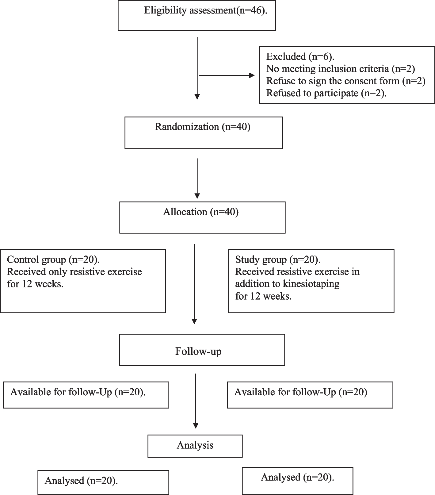
Fig. 1
Steps of conducting the research
Dataset collectionIn the present case–control study, DLBCL data was used, which included 180 genes expression and 31 individuals. The data is available on the following site: https://www.ncbi.nlm.nih.gov/. The dataset includes blood samples from 31 donors, including 14 healthy individuals and 17 DLBCL patients. The notable point about the dataset is that when donating blood, people have no symptoms of the disease and are healthy enough to donate blood. According to Jorgensen et al., this is the first study of the microarray expression profile of apparently healthy individuals taken several years before the diagnosis of DLBCL [11].
Gene selectionAccording to the dataset of the study, the most appropriate regression models were processed on these data. Regression models include the Ridge, the Lasso, the Elastic Net, and the Precision Lasso.
Shrinkage regression modelsWhen the number of variables p is greater than the number of observations (p ≫ n), the ordinary least square method cannot be used to estimate linear regression coefficients. Another issue is determining the number of independent variables that should be used in the model. As the number of variables increases, over-fitting occurs, and as they decrease, we may encounter under-fitting.
To solve the problem of estimating parameters in high-dimensional data in the last two decades, many methods were proposed based on the dimension reduction and the converted minimum squared error estimator. Here, four different penalty methods are described with their advantages and disadvantages.
Ridge regression modelThe best way to estimate the regression model parameters, due to the lowest error, is the ordinary least square method. However, it cannot be expected minimum variance for the estimators. Therefore, we need to find a way to select the right number of estimators. The application of Ridge regression is clarified in such situations. The estimator of Ridge regression is not unbiased but has a smaller variance than the ordinary least square method. In the ridge regression model, using the constraint ∥β∥2 ≤ C 2 on the parameters of the regression model, it tries to fix or reduce the sum of the squares of the parameters, so this constraint was added by the ordinary least square method.
One of the features of the Ridge regression model is that the penalty function reduces the coefficients to zero but does not make any of them zero. Of course, this does not apply to a so large λ. This feature challenges the interpretation of a model with a large number of variables [9].
Lasso regression modelThe Lasso regression model provides a suitable method for modeling the response variable based on the lowest and most appropriate number of explanatory variables. This method separates the more suitable variables from the rest of the variables by providing a simpler model. That is why it is known as the Lasso method, which is a Canadian word meaning snare. In 1996, Robert Tibshirani, by using a penalty function on the sum of the absolute values of the regression model coefficients, controlled the number of parameters. In this condition, the sum of the squared estimate of errors of the Lasso model writes as follows:
$$\sum\nolimits_^ \left( y_ - \beta_ - \sum\nolimits^_ \beta_ x_\right)^ + \lambda \sum\nolimits_ \left| \beta_ \right|$$
(1)
λ is a regulating parameter, meaning that if its value is zero, the model will become linear regression, and all variables will be present in it. If its value increases, the number of explanatory variables in the model will decrease. One of the main goals of the Lasso is to improve the interpretation of the model by determining a smaller subset of explanatory variables that have the most effect [7].
Elastic Net regression modelThe Elastic Net regression model was introduced by Zu and Hasti. Elastic means flexibility. In fact, the Elastic Net model is a combination of Lasso and Ridge models and uses second degree penalties. This method is used when the Lasso cannot select the grouping variable by one category and ignore the other categories. Using this model can be useful for the dataset with high correlation [10].
Precision Lasso regression modelThe regular regression model, introduced by Wang et al. as Precision Lasso proved the instability and inconsistency in the Ridge, Lasso, and Elastic Net models primarily by using a condition called irrepresentable. The condition is as follows:
$$\left|^\right)}^^^\right)}^^\right)}^sign\left(^\right)\right|<1-\eta$$
(2)
In this condition, x (1) is a set of active variables x (2) is a set of inactive variables and η is a positive constant vector.
The instability of the Lasso points to its inability to detect the effects of correlated explanatory variables. Since correlated explanatory variables cannot analyze separately and by classical statistics, a simple way to achieve this goal is to determine similar weights for correlated variables. Considering the Trace Lasso regression model, a set of weights in which the correlated variables add to the other variables. Inconsistency is another disadvantage of the Lasso, which refers to the collinearity between variables. To solve the two problems of instability and inconsistency, for the first time, Wang et al. proposed γ a regulatory parameter to combine the two solutions. However, for example, if there is instability, γ = 1, and if there is inconsistency, γ = 0, and if there are both of them, γ = 1/2. The strategy introduced can be extended to other ℓ functions more simply. As an example, when the Response variable is dichotomous, by substituting ℓ with the negative in the likelihood logarithm, the Precision Lasso model is converted into a logistic regression model. This formula is applied in case–control data as those in the present study.
$$arg\ min\ell\left(x,\gamma ;\beta \right)+\lambda \Vert \left[^x\right)}^\frac+\left(1-\gamma \right)^x+\mu I\right)}^}\right]diag\left(\beta \right)\Vert$$
(3)
In the present study, due to the high correlation of genetic data, we tried to find cancer-related gene markers using the above four penalty methods [8].
Model evaluationWe evaluated shrinkage regression models using two steps. In the first step, according to previous studies, the expressed genes caused by DLBCL disease were identified. Then, we compared the genes that were selected using the models with the identified genes. In the next step, the holdout method was used with 10 folds. Then, the goodness of fit of regression models was compared based on the area under the ROC curve (AUC) and average precision score (AP-Score) [12].
Analysis of gene expression data was performed using R 3.6.2 and Python 2.7 software.
留言 (0)