

Remember me


A key property of HE is the relationship between the probability density function (the brightness histogram normalized to sum to 1) of an input image and the tone curve used for enhancement. The latter is the cumulative histogram—equally, the integral—of the former.
Now, returning to our example in Figure 1, suppose H() is the tone mapping function—from HE—that resulted in a poor image reproduction. There were areas where contrast was too high and others where it was too low. Let us suppose there exists a better tone mapping function, G(). From our previous discussion, by differentiating the G(a) we can return a density function g(a). It turns out that finding G(a) can be usefully expressed as the problem of finding g(a) given h(a). The aim is to find a g(a)—as a proxy for h(a)—that would integrate to a better tone map.Let us choose g(a) to be close to h(a), but where its individual densities are neither too large nor too small. It follows that the corresponding tone curve—defined to be the integral of the density function—must have a bounded slope. This intuition is the central idea underpinning Contrast Limited Histogram Equalization (CLHE) [3], a widely deployed tone mapping algorithm. Importantly, CLHE also underpins the Apical Iridix tone mapper [15] that is embedded in many cameras and smartphones.In Figure 1b, the red dotted line shows a probability density close to the original (solid blue line) but has a bounded density (in this example it is between 0.02 and 0.005, where the brightness range is divided into 100 bins). The corresponding cumulative histogram is shown in Figure 1f. Notice how the maximum slope is reduced and the minimum slope increased. Finally, in Figure 1e, we show the CLHE output. Here we have good detail throughout the image and a pleasing reproduction where the image detail is rendered to be more conspicuous.The first contribution of this paper is to show that each iteration (refinement) of the CLHE algorithm can be represented as a special tone mapping computational block in a neural network (where the internal structure—the connections—of the block are derived in Section 3). Of course unrolling iterative algorithms by means of a Neural Network is an established approach to accelerating iterative algorithms [16]. The important distinction here is that representing CLHE as a computational block lets us pre-define the parameters of the network (as opposed to random initialization). It will be shown that a deep net of a sufficient number of repeating layers exactly computes the CLHE histogram modification. We call the deep net that comprises repeating tone mapping layers a Tone Mapping Network, or a TM-Net for short. We illustrate the idea of unrolling an iterative histogram refinement algorithm by an equivalent TM-net architecture, in Figure 2.In Figure 2a, we show the high level view of the CLHE algorithm that maps an input brightness density, h0(a) to the output density g(a), where ultimately, the tone map will be defined as the integral of the latter.We describe the function computation() in the next section and its implementation as a neural computational block in Section 3. In each iteration, the density hi(a) is refined from hi−1(a). The iteration terminates when a convergence criterion is met.On the right hand side of the Figure 2b, the solid blue vertical bars denote input and output densities (e.g., vectors of numbers). Inputs and outputs are connected by a network of connections. In the usual neural network way, each connection line takes an input value (one bin of the input histogram/density) and multiplies it by a weight. Per bin on the output layer we sum across all the connections (that input to that bin). The network connections shown here are for illustration only. The precise connectivity follows from the CLHE algorithm (and this is discussed in detail in Section 3). In the usual neural net way, the output layer feeds through an activation function, here piece-wise linear. Importantly, the piece-wise linearity follows exactly from how CLHE enforces height constraints on the probability densities.So long as the network we define is built with a sufficient number of computational layers—as illustrated in Figure 2c—then the resulting deep net calculates exactly the same output as CLHE. The architecture shown in Figure 2 is called a tone mapping network, or TM-Net for short. Importantly—and unlike typical networks—our unrolling of CLHE here ensures the layers of the TM-Net are interpretable.Of course, all we have done at this stage is re-represent an existing computation in a different form. In this paper we will also use our TM-Net architecture to make CLHE faster to compute, and also to compute tone maps that make images that are preferred to CLHE. In the second contribution of this paper, we replace our 60+ repeating block architecture with a simple 2-layer TM-Net. However, now, rather than adopting the default CLHE weights, we relearn them in the usual deep learning way (by Stochastic Gradient Descent [17]). The loss is determined by the difference between the 2-layer TM-Net output and the iterated-to-convergence CLHE output. We therefore seek—in just 2 layers—to compute the same output histogram as CLHE computes (in the worse case 60+ iterations). Effectively reducing the number of iterations allows us to overcome one of the primary drawbacks of CLHE, it is unpredictable and often significant computation time [18,19].Of course, there are many other algorithms that determine a tone map dependent on the histogram of an image. So, in our third contribution we aimed to see whether our TM-Net could be used to learn non-CLHE tone maps. Here, we chose to investigate the algorithm of Arici et al. [20] both because it produces pleasant images, (often preferred to CLHE) and also because it has quite a complex formalism (including, in its general form, using quadratic programming). We found that we can retrain the TM-net to learn the outputs computed by [20], and in so doing make that method simpler to implement and faster to execute. Importantly, our TM-Net we define here is used to closely approximate (and speed up the execution for) existing algorithms, that is, we are not designing new tone curve algorithms here.In Section 2 of this paper, we review the related background work. Our TM-Net is derived and presented in Section 3. In Section 4 we show—based on a large corpus of images—that a 2-layer TM-Net can be used to implement CLHE (which by default can take 60+ iterations to converge) thereby making it a much faster algorithm. We also demonstrate that the more complex tone mapper (from Arici et al) can also be implemented as a TM-Net. The paper concludes in Section 5. 3. MethodThe starting point of this paper is to re-cast the CLHE algorithm into a form that we call a Tone Mapping Neural Network or TM-Net for short. Abstractly, the TM-Net implements each iteration of the CLHE algorithm as a single layer in a network computation, see Figure 2. Crucially, the network architecture and all the weights are defined by the CLHE algorithm (at this stage there is no learning). By building a deep net by repeating these layers we make an architecture that exactly calculates CLHE.By translating an iterative algorithm to an equivalent deep net, we can ask new and novel questions. First, can we improve the speed efficiency of CLHE? Specifically, can we use a TM-Net with 2 layers to learn the CLHE computation? Secondly, can we use the TM-Net to learn other histogram-based tone-mappers?
3.1. The TM-NetIn Equation (1), we summarized the key components of a Neural Network layer. The 4 components include 2 known and 2 unknown variables. The known variables are the output of the previous layer in the network (al−1), and the activation function (σ()). The unknown variables are the weight matrix (wl) and bias vector (bl). Training a Neural Network means that we need to solve for wl and bl that map the input vector to a desired output (al). In this section, we marry CLHE and Equation (1), i.e., we derive the matrix, bias vector, and activation function that—when used in Equation (1)—would generate an output vector that exactly matches one iteration of CLHE.We start with the observation that the clipping step of CLHE (Equation (9)) is analogous to the role of an activation function in a Neural Network and so the transcription is natural. Indeed, a simple piece-wise linear function [36] is illustrated in Figure 4a that computes the clip in Equation (9) and step 4 of the CLHE algorithm. The function is linear on the interval [L,U], and flat everywhere else. Here, L and U denote the lower and upper slope bounds (clip limits) respectively. When this function is applied to the histogram in Figure 4b we find the ‘clipped’ histogram in Figure 4c.The redistribution step of CLHE is visualized in Figure 5. We will conceptualize the redistribution process as two separate steps. First, we consider how to add an offset so a histogram sums to zero, Figure 5b. Given a zero-mean histogram, we can add the offset (1N to each bin) in Figure 5c to make a histogram that sums to 1. This two step view makes the redistribution step simple to write in matrix form.Let us define the N×1 vectors v and w where vi=1 and wi=1N (i=1,2,⋯,N). Remembering that our N-bin histogram is denoted h and denoting the N×N identity matrix by I, we calculate: which, effectively, adds the same value to each component of h so that the resulting histogram sums to 0 (we use the superscript 0 to denote the histogram has a zero mean). Now we add the second offset. We define a fixed N-vector b where each component bi=1N. Using the piece-wise linear function from Figure 4 as σ(), we can now express the histogram found by i+1 iterations of CLHE, hi+1, as:hi+1=[I−vwT]σ(hi)+b
(17)
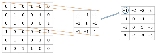
Returning to Equation (1) we are ready to transcribe the CLHE into a network computation. For σ() we use the piece-wise linear function in Figure 4 with bounds at the desired clip limits. The wl weight matrix is calculated as I−vwT as defined above. Additionally, bl is a vector that holds 1N in each element.Our transposition from matrix equation to a Neural Network layer is further illustrated for a 5-bin example in Figure 6. Weighted connections between bins are represented as arrows (initialized to the shown values). From left to right, the input to the network first passes through the piece-wise linear clipping function. Next, the dashed orange and green lines represent multiplication of the input by v and wT respectively, which is fed into the output layer. The input layer also feeds directly into the output layer, and—along with the bias vector (b)—the sum of all components define the output. This output—depending on the network architecture—is either fed into the activation function again, or is the network output.Figure 6 shows that each iteration of CLHE can be thought of as a standard type of neural net computational block, where the input histogram is mapped to an output version by a matrix operation plus a bias, that is then rectified by a piece-wise linear function. Clearly, if we repeat the block structure enough times then the network must, by construction, calculate the same answer as CLHE. That is, if the conventional CLHE algorithm takes m steps to converge then the same answer can be found by replicating m layers of the form shown in Figure 6. In our experiments, we found CLHE always converged in 60 iterations or fewer (mostly in less than 20 iterations). So, we need a 60 layer deep TM-Net to guarantee the same result as CLHE (to numerical precision). We call our repeating block architecture a Tone-Mapping Network or TM-Net for short.Finally, we note that, as the block is drawn, it actually resembles a residual neural network (albeit a very simple one). The actual computation is a simple summation followed by a propagation of the sum (follow the red and green dotted arrows). Then we add in the results from a previous layer.
3.2. Relearning CLHEWe hypothesize that a small network can be initialized (fewer layers than needed for CLHE convergence) to use a truncated TM-Net to learn the result of the fully convergent CLHE operation. Our hypothesis is that a truncated TM-Net with learned weights (we do not use the defaults that follow from the CLHE algorithm) will be able to learn the CLHE computation.
To be more concrete, suppose we have a network that has m layers built as described in the last section, and let us denote the output of a TM-Net as TM(h). For the ith histogram in a dataset the network computes TM(hi) We would like the network to produce histograms that are similar to the CLHE computation, CLHE(hi), i.e., we would like TM(hi)≈CLHE(hi).
Suppose we use m computational layers of the form shown in Figure 6. In the kth (of m) computational block we have to learn 3N unknowns which we denote vk, wk and bk. Grouping the complete set of all the unknown v’s, w’s and b’s as the N×m matrices V, W and B (each column of each matrix is respectively v, w and b). Then for an m-layer network we need to minimizeJ=minV,W,B∑i||CLHE(hi)−TM(hi)||2
(18)
where the Equation (18) is a simple least-squares loss function. It is implicit that to minimize Equation (18) that we need to find V, W and B (the network parameters) that makes the squared error as small as possible. In fact we would also like to place some constraints on these hidden variables. Given that vi—a set of network weights—is weighting a histogram, and a histogram has a natural order (bins range from a brightness level of 0 to 1 in increasing order) we would like vi to be smooth in some sense. The intuition here is that we do not expect the kth weight wkl to be significantly different from wk+1l. That is, the weights and bias vectors, vl, wl, bl, (usefully visualised as functions plotted on a graph) should be smooth. Here we define the smoothness of all the parameters asS=(||DV||2+||DW||2+||DB||2)
(19)
where D is the N×N linear operator that calculates the discrete derivative (of a column vector), e.g., see [20]. In Equation (20) we set forth the final form of our minimization (where λ is a user defined parameter weighting the importance of the smoothness of the network parameters). The weights and biases—underpinning the optimization in Equation (20)—can be found by Stochastic Gradient Descent (SGD) implemented using back propagation (BP) algorithm. The details of the SGD and BP algorithms (e.g., [17]) are not important here. What is important is we can optimize Equation (20) efficiently using standard techniques. By minimizing Equation (20) we relearn CLHE. 3.3. Training the Truncated TM-Net (Implementation Details)We use a TM-Net with as few as two layers to approximate CLHE. The network was trained using 30,000 images randomly samples from the ImageNet dataset [37]. From each training image, we obtain the input histogram and the CLHE histogram (the network does not see the full image, only the histograms). These histograms serve as the input and target of the network respectively. The network was trained using the regularized mean squared error loss function (in Equation (20)) with λ = 1×10⁻⁴ and the following hyper parameters: batch size = 30,000, learning rate = 1×10⁻⁴, and epochs = 500. The machine used for training uses PyTorch and an Intel i7 CPU and an NVIDIA RTX 2070S. Each training epoch resolved in 0.75 s for a total training time of 6 min.As we will show in the experiments section, we also train networks (with the same hyper parameters) with more than 2 layers.
3.4. Cost of Learning and Applying a Tone MapOur method—like CLHE—generates a tone curve from the histogram of brightnesses in an image. To build this histogram we need to visit each image pixel once. Once we have calculated the tone curve then to apply this curve we again need to visit each pixel once. Thus the cost of CLHE and our variant is proportional to the number of pixels in the image. However, the actual cost of calculating the tone curve is constant (independent of the size of the image).
4. ExperimentsWe evaluate the performance of our TM-Net by comparing the closeness of images enhanced with the TM-Net against two target algorithms: CLHE [3] and the Histogram Modification Framework (HMF) [20].Effective comparison of images is a challenging problem [38]. Here, we use the ΔE distance metric to quantify closeness of the enhanced images. This was a deliberate choice because the tone curves used in this work are applied globally to each image. We also ran tests using the SSIM (structural similarity measure) and PSNR (peak signal to noise ratio) and found the results to follow the same trend as the ΔE errors (and so are not reported here). That said we include, for completeness, SSIM and PSNR results for the most challenging dataset.To calculate ΔE error statistics, each test image is enhanced with the target algorithm, and then enhanced independently with the TM-Net tone curve. Each enhanced image is then converted to the CIE L*a*b* colour-space, and the per-pixel difference of respective channels in each image is calculated to generate an error image. From this error image here, we calculate the mean, median, and 99-percentile error statistics for the input image, and do this for all images in the test datasets.
To be precise, the mean statistic is the mean of the individual means calculated per image. Similarly our median statistic is the median of the median errors again calculated per image. Similarly, for a given image we can calculate the 99-percentile CIE L*a*b* ΔE error. Then over a data set we can calculate the 99-percentile of the 99-percentile errors.
In our experiments, we will use four test datasets in this work. The well-known Kodak dataset [39] that contains 24 RGB images comprises our first image set. Remembering that 30,000 images from Image Net is used to train our TM-NET, the remaining 20,000 RGB images (not used for training) are used as our second image test set. [37]. In our third image set, we use 20,000 RGB images from the MIT Places database [40]. Our 4th image set draws challenging images from the first three datasets. Challenging examples are images that take more than 45 iterations for CLHE to converge. 4.1. Approximating CLHE: Contrast Limited Histogram EqualizationHere we wish to use our TM-NET to approximate CLHE. We will compare the outputs of the TM-Net according to our mean, median and 99-percentile statistics over our four image sets. In all cases, we found that the TM-Net always well approximated CLHE in three or fewer layers (and so we will only consider these approximations here).
In Figure 7, from left to right, we plot the mean of the mean, median of the median, and 99-percentile of the 99-percentile of ΔE for each of the test datasets used in this work, as a function of the number of layers in the TM-Net. We see that while the error in all instances is not 0, it is indeed close to 0 and, naturally, becomes closer to 0 as the number of layers in the TM-Net increases. A common heuristic approach to determining the point of diminishing returns is to identify the ‘elbow’ of the error curve. For all examples in the figure the elbow occurs at two layers.Moreover, in complex images (e.g., photographic pictures like the ones used in this work) an average ΔE—where the error is distributed throughout the image—of between 3 and 5 [41,42] is generally thought to be visually not noticeable. For our data, this—like the elbow—points to a 2-layer TM-Net sufficing.In the first three results columns of Table 1, we compare the performance of a 2-layer TM-Net against fully converged CLHE. Notice the mean of the mean ΔE is close to zero (visually indistinguishable in most cases). Significantly, for the most challenging images, the 99 percentile error is just 3.09 which is visually not significant for complex images. The final column in the table reports the 99 percentile ΔE error for the 2-iteration CLHE (hrer, we manually limit the permitted number of iterations to 2). Notice that for the first 3 rows/datasets the errors for 2-iteration CLHE are fairly low (though higher than the 2-Layer TM-Net approximation). This is because in most cases CLHE converges in few iterations. However, for the challenging dataset, the 99 percentile ΔE error is 5.81 (significantly larger than the TM-Net approximation and visually noticeable).In Figure 8, we present an example of an output generated using an image drawn from the challenging dataset. We compare the output of the fully converged CLHE with the 2-layer TM-Net. As expected from the error stats presented, the outputs are visually identical. For comparison, we also run CLHE but terminate it, arbitrarily, after two iterations. Here, there is a significant residual difference. Pay close attention the image outputs corresponding to the input region bounded by the red rectangle.In Figure 8 (right), we show the input histogram and the modified histograms for the three algorithms. We see that the TM-Net output is almost identical to CLHE iterating to convergence. However, the 2-iteration CLHE has a noticeable delta.Additionally, we highlight the differences between the 2-layer TM-Net (left) and 2-iteration CLHE (right) outputs with a heat-map of ΔE in Figure 9. The colours in the figure moving from blue to yellow represent increasing difference between the output images from the target image. The erroneous pixels for the limited CLHE error image cluster around the diver. The mean of the mean ΔE error for the TM-Net and limited CLHE outputs are low, 1.1 and 1.9, respectively. While the 99-percentile of the 99-percentile ΔE error tells us the same respective difference is 2.6 and 3.9. Clearly, the TM-Net output is much closer to the target.Finally, in Figure 10 we show several images from the Kodak dataset (left) enhanced with full-iteration CLHE (middle) and the 2-layer TM-Net (right). The ΔE for each image in the set is shown in the top right. The mean ΔE error is close to 0 for all images and there are close to zero noticeable differences even under very close observation. 4.2. HMF: A Histogram Modification FrameworkThe original Quadratic Programming (QP) based implementation of HMF is complex (see Equation (12)). Here, we seek to reformulate the algorithm into the proposed TM-Net form. Essentially, we ask if this more complex algorithm be made as simple as CLHE. To retrain the TM-Net, we use the same architecture and training dataset as the CLHE TM-Net, and extract from each image the original and HMF modified histograms. As before, we can summarize our network with Equation (18)—replacing CLHE(hi) with HMF(hi)—and also including the smoothing constraints on the parameters of Equations (19) and (20). As before, we initialize the parameters (weights) of the network to the CLHE weights.In Table 2, we compare the performance of our bespoke 2-layer TM-Net against the Histogram Modification Framework [20]. Clearly, the ΔE is not zero, but the numbers are small. As for approximating CLHE, a 2-layer TM-Net suffices to approximate the HMF framework. 4.3. PSNR and SSIMWe present Peak Signal to Noise Ratio (PSNR) and Structural Similarity Index Measure (SSIM) statistics for the challenging images dataset in Table 3. To obtain these statistics, we used MATLAB’s respective ssim and psnr functions to compare the TM-Net reproductions against the respective CLHE and HMF reproductions. The final row in the table compares the CLHE TM-Net against 2-iteration CLHE. Mean PSNR and SSIM results are shown and their standard deviations.Figure 10. For each image in the set: First, original image. Middle, image enhanced with CLHE. Right, image enhanced with a 2-layer TM-Net. Mean of mean ΔE between the enhanced images are shown in top right of each image.
Figure 10. For each image in the set: First, original image. Middle, image enhanced with CLHE. Right, image enhanced with a 2-layer TM-Net. Mean of mean ΔE between the enhanced images are shown in top right of each image.
For the 2-layer TM-Net approximation to CLHE, both the PSNR and SSIM results show that the 2-layer TM-Net delivers a better approximation to the full CLHE algorithm compared to running CLHE for two iterations. The PSNR is 47.52 for the 2-layer TM-Net but only 38.13 when CLHE is run for two iterations. Analogously, the SSIM (where 100 means perfect similarity), the mean SSIM for the 2-layer TM-Net is 0.97 and 0.95 when CLHE is run twice.
4.4. Execution Time of CLHE vs. TM-NetFinally, we compare the speed of the TM-Net compared to CLHE. Since the tone curves here are applied to images in exactly the same way, when we measure timings we only consider the execution of the histogram modification steps (and not the application of the tone curve to images). In the introduction, we stated CLHE in the worst case we found converges in 60 iterations, and our TM-Net has two layers, thus from the perspective of modification steps the TM-Net is up to 30 times faster.
Next, we measured our MATLAB implementation of CLHE on the ImageNet and Places datasets (40,000 images total). The total computation time was 1063 s, or 26.6 ms per image. The TM-Net on the same dataset converged in 712 s, or 17.8ms per image. That is, running CLHE on the dataset took 49.3% longer. These timing experiments were performed on a machine running an Intel i7 CPU and an NVIDIA RTX 2070S.
5. ConclusionsContrast Limited Histogram Equalization (CLHE) [3] is a widely used tone adjustment algorithm that ships in cameras and smartphones (including, the Apical IRIDIX algorithm [15]). CLHE is an iterative algorithm which iteratively refines a histogram so that its cumulative distribution (which defines the CLHE tone curve) has bounded slope (neither too small nor too large). In our experiments, we found that CLHE often converged quickly but that it was not unusual for it to take 20 iterations or, in the worst case, 60 iterations to converge.In this work, we show how CLHE can be exactly transcribed into a neural network framework that we call TM-Net. The TM-Net has as many layers as there are iterations in CLHE with the weights in the network prescribed by the CLHE algorithm.
That we define CLHE as a neural network allows us to take advantage of the fact that a network can learn new parameters. That is, we need not use the weights that follow from the CLHE algorithm but we can relearn them in the usual network learning manner, i.e., by stochastic gradient descent. Surprisingly, we show that the outputs from a 2-layer TM-Net visually approximate the images generated by the CLHE algorithm running to convergence. The 2-layer TM-Net always runs much faster than the CLHE algorithm that it approximates.
Next, we were interested whether our TM-Net architecture could be used to learn other tone mapping algorithms. To test this idea, we took the Histogram Modification Framework (HMF) [20] as an exemplar algorithm. The general HMF framework finds a tone curve with an optimization defined as Quadratic Program. In HMF, various objective functions are minimized, including terms that ensure the tone curve maps, respectively, blacks to blacks and whites to whites, and that the tone curve should be smooth. Significantly, overall the HMF framework produces preferred tone-renderings to CLHE.Again, we find that a trained 2-layer TM-Net is able to well-approximate HMF. Here the efficiency gains are even more stark. Quadratic Programming is an expensive algorithm to implement and run. Implemented as a 2-layer TM-Net, the complexity of HMF is found to be no greater than CLHE.
Comments (0)