1 Introduction

Compressed sensing (CS) can simultaneously sample and compress signals, and accurately reconstruct the original signal from the sampled data. Once proposed, this theory has attracted widespread attention in the academic community. In order to reduce the amount of information collected by wearable ECG devices, compressed sensing technology is used to simultaneously collect and compress signals, which greatly reduces the amount of collected data, improves the energy efficiency of wearable devices, and has been widely used. Balouehestani et al. (2013) combined CS with block sparse Bayesian learning (BSBL) theory for wireless ECG acquisition, significantly reducing the sampling frequency and power consumption; Zhang et al. (2013) used CS and BSBL for remote monitoring of fetal ECG, also with the aim of reducing the sampling frequency and power consumption; Shoaran et al. (2014) used CS for the biomedical signal acquisition system of sensor arrays, which not only reduced power consumption and data volume, but also reduced the area of electrodes. Reconstructing the original signal from the compressed data is one of the core research contents of compressed sensing technology.

Reconstruction algorithms based on compressed sensing technology can be divided into three categories: (1) Convex optimization algorithms (Liu et al., 2017), which transform NP-hard ℓ0 norm problems into convex optimization problems with ℓ1 norm. (2) Greedy matching pursuit algorithm (Nguyen et al., 2017), a greedy optimization algorithm that selects the most suitable atom in each iteration based on the greedy strategy and adds it to the candidate set. (3) Bayesian reconstruction algorithms (He et al., 2010), transforming the reconstruction problem into a probability-solving problem by utilizing the prior probability distribution of the signal.

Approximate message passing (AMP) (Donoho et al., 2009), a reconstruction algorithm based on iterative thresholds, is particularly suited for real-time reconstruction in scenarios where signals such as electrocardiograms (ECGs) require rapid and efficient processing. However, the design of filters and their ability to exploit signal structure characteristics, based on AMP reconstructions, significantly impact reconstruction performance. During the research process, scholars have imposed constraints on the prior information inherent in the signal, proposing various forms of denoising models, including sparsity priors, gradient priors, non-local self-similarity priors, and low-rankness priors.

Based on the sparsity prior of images, Som (2012) employed wavelet transforms in conjunction with hidden Markov trees (HMT) for modeling and reconstruction, thus reducing computational complexity while enhancing reconstruction performance. Tan et al. (2015) applied the wavelet-domain adaptive Wiener filter to the AMP framework and proposed the AMP-Wiener algorithm. Hill et al. (2016) designed an AMP algorithm based on the Cauchy prior in the wavelet domain, which converges about twice as fast as the AMP method and improves the reconstruction quality. However, wavelet sparsity is not suitable for non-stationary natural signals. The gradient sparsity prior, which better preserves edges and textures, has attracted scholars’ attention. Wang and Liang (2015) proposed an AMP algorithm that utilizes the gradient sparsity prior to preserve image edges and texture information.

Another research direction for signal denoising is designing denoising operators that match the sparse characteristics of the target signal, where dictionary learning-based denoising is an efficient technique (Xu et al., 2021; Xue et al., 2020). The research results indicate that dictionary learning algorithms such as K-SVD (K-means singular value decomposition) (Aharon et al., 2006; Scetbon et al., 2021) and SGK (sequential generalization of K-means) have better denoising performance than denoising algorithms based on wavelet domain. Li et al. (2017) proposed a dictionary learning based AMP (DL AMP) algorithm, which integrates dictionary learning methods into the AMP algorithm to achieve denoising and achieve better image reconstruction performance than fixed transform domain denoising operators. The disadvantage is that the DL-AMP algorithm needs to train the dictionary in each iteration, and the training data entirely from the current signal to be filtered, and the number is very limited, which limits the denoising performance of the algorithm. At the same time, the dictionary training process is time-consuming, resulting in longer runtimes for DL-AMP.

The above research methods only utilize the local features of the signal, but ignore the non-local information contained in a large number of similar blocks in the signal. Metzler et al. (2016) proposed the denoising-based approximate message passing (D-AMP) algorithm, which incorporates a block-matching and 3D filtering (BM3D) denoiser (Dabov et al., 2007) that utilizes image non-local similarity priors during each iteration of the filtering process, thereby enhancing reconstruction performance. However, using non-local similarity prior requires searching for similar image blocks. The common criterion for measuring similar blocks is Euclidean distance. In the presence of noise, noise can affect the calculation of similarity between image blocks, causing a higher similarity scores between dissimilar blocks, thus impacting denoising performance.

In order to further improve reconstruction performance of compressive sensing, this paper proposes an improved weighted nuclear norm minimization algorithm for approximate message passing algorithms. In the presence of noise, dissimilar signal blocks may be grouped together, resulting in a signal block belonging to different similar block groups, so that the misclassified signal blocks obtain different denoising effects. Therefore, the weighted nuclear norm minimization (WNNM) algorithm, which averages the signal blocks after low-rank decomposition, is not suitable for obtaining the denoised signal. Theoretically, the greater the similarity between signal blocks, the lower the rank of the similar block group matrix, and the better the denoising effect. However, misclassified signal blocks will affect the low rank characteristics of the similar block group matrix, resulting in poor denoising effect. If each signal block is directly averaged to obtain the denoised signal, the details may be smoothed. Therefore, the denoised signal should be the weighted average of multiple signal blocks. Based on this, this paper improves the WNNM algorithm by proposing to use weighted averaging instead of direct averaging for the signal blocks after low-rank decomposition in the denoising process.

2 The background introduction 2.1 D-AMP algorithm

The mathematical model for compressive sensing can be expressed as:

y=Φ⁢x(1)

Signal x ∈ RN represents the original electrocardiogram signal, Φ ∈ RM×N(M ≪ N) is the observation matrix, and y ∈ RM is the obtained observation value. That is, the original ECG signal x is projected onto the low-dimensional space through the observation matrix Φ to obtain an M dimensional observation signal.

The DAMP algorithm reconstructs vector x ∈ RN based on the vector y and the measurement matrix Φ.

xt+1=Dσ^t⁢(xt+ΦT⁢zt)(2)

zt=y-Φ⁢xt+zt-1⁢Dσ^t′⁢(xt-1+ΦT⁢zt-1)/M(3)

σ^t=||zt||2M(4)

Where xt is the t-th iteration estimate of the original signal x0, zt is the residual, σ^t is the standard deviation of the noise, xt + ΦTzt is equivalent to the superposition of the original signal x and Gaussian noise, Dσ^t⁢(•) represents the denoising operator acting on xt + ΦTzt, making the output xt closer to the original signal x than xt–1, and Dσ^t′ is the derivative of the denoiser. The denoiser plays a key role in the D-AMP algorithm, directly affecting the quality of signal reconstruction and determining the algorithm’s reconstruction performance.

2.2 The weighted nuclear norm minimization (WNNM) algorithm

ECG signal denoising is the process of removing noise from noisy ECG signals and restoring the original ECG signals. Let q = x + n where q is the noisy ECG signal, x is the original ECG signal without noise, and n is the noise. The ultimate goal of ECG signal denoising is to obtain an estimated value x^ of the original ECG signal, where x≈x^.

The WNNM algorithm utilizes the similarity of signal structures and applies soft-thresholding shrinkage to singular values with different values, achieving good denoising effects. Given a noisy ECG signal q, let qi be a local signal block of q. By using block matching algorithm to search for non-local similar blocks to form matrix Qi, let Qi = Xi + Ni, where Xi is a matrix block of the original ECG signal without noise and is a low-rank matrix, Ni is a noise block. The objective function of WNNM can be expressed as:

X^i=arg⁡minXi⁡1σn2⁢||Qi-Xi||22+||Xi||w,*(5)

Where σn2 is the noise variance used to normalize the Frobenius norm, ||Xi||w,* = ∑i||wjσj(Xi)||1, σj(Xi) represents the j-th singular value of Xi, and each item in w = [w1, w2, …, wn] is a non-negative number, corresponding to each singular value, as follows:

wi=c⁢d/(σj⁢(Xi)+ε)(6)

σj⁢(Xi)=max⁡(σj2⁢(Qi)-d⁢σn2,0)(7)

Where, σj(Xi) is the j-th singular value of Xi. It can be observed that the larger the singular value, the smaller the weight. c is a constant greater than 0, dis the number of similar blocks, and ε is a small parameter to prevent division by zero. Perform singular value decomposition on Qi,Qi = UΣV.

ςw⁢(Σ)=max⁡(Σii-w,0)(8)

Where, Σii is the diagonal element of the singular matrix Σ, so the solution of the objective function is obtained:

Xi=U⁢ςw⁢(Σ)⁢V(9)

3 Proposed method 3.1 Improved weighted nuclear norm minimization algorithm

The WNNM algorithm has achieved good denoising results. However, when searching for non-local similar blocks, there is a possibility of misclassification by measuring the similarity of two signal blocks using Euclidean distance, which may result in grouping dissimilar blocks together and affecting the denoising effect.

In the presence of noise, the similarity between signal blocks qi and qj can be expressed as follows

Dqi⁢qj=(xi-xj)2+(ni-nj)2+2×(xi-xj)×(ni-nj)(10)

Where, qi = xi + ni, qj = xj + nj.

In formula (10), (xi − xj)2 is the distance obtained by the noise-free signal block, which is the real similarity of the signal block. (ni −nj2 + 2 × (xi − xj) × (ni − nj) is the error caused by noise, which may cause the Euclidean distance between signal blocks that originally have no similarity to be smaller, thus dividing them into a group. Since dissimilar signal blocks lack structural and data similarity, the resulting matrix is not a low-rank matrix, and averaging over each signal block is not suitable for denoising in the WNNM algorithm. In theory, the larger the similarity between similar blocks, the lower the rank of the matrix, Therefore, the denoised signal should be the weighted average of the signal blocks. Based on this, an improved WNNM (IWNNM) algorithm is proposed.

Xi=1m⁢(i)⁢e-rl⁢Ai(11)

Where m⁢(i)=∑ie-rl, r is the rank of the matrix ςw(Σ) and l is the number of rows in the matrix Qi. Ai = Uςw(Σ)V The ECG denoising process based on IWNNM is shown in Figure 1.

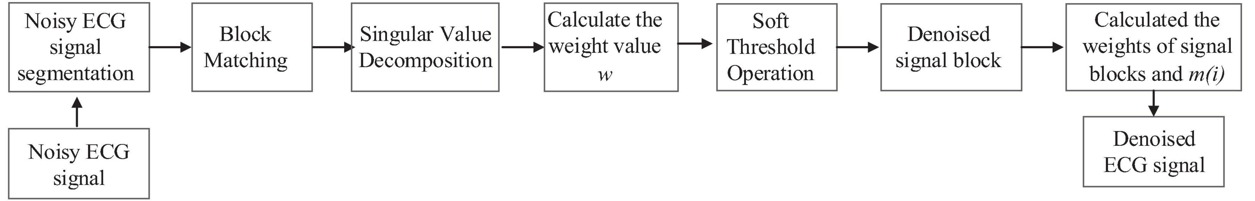
Figure 1. Flow chart of ECG denoising based on IWNNM.

Firstly, the noisy ECG signal is divided into blocks. One block is selected as the reference block, while the others are candidate blocks. The block matching algorithm is used to find similar signal blocks from the candidate blocks compared to the reference block. These non-local similar blocks are arranged as column vectors to form a group of similar signal blocks. Through singular value decomposition, soft thresholding operation achieves low-rank matrix approximation, obtaining denoised signal blocks. During the process of singular value decomposition, different weight values are assigned to signal blocks based on the rank of similar signal block groups. The denoised signal is obtained by taking the weighted average of the denoised signal blocks. The denoising process of the IWNNM algorithm is shown in Algorithm 1.

Algorithm 1. Improved WNNM (IWNMM) algorithm denoising process.

Input noisy signal q, number of iterations K

Initialize x^0=q,q0=q

for t = 1:K do

Regularize qt=x^t-1+δ⁢(q-q^t-1), and divide vector qt into different signal blocks.

For each sub-block qi do

Find its similar sub-block group Qi.

Singular Value Decomposition[U,Σ,V] = svd(Qi)

Where Ai = Uςw(Σ)V

Estimate obtained: Xi=1m⁢(i)⁢e-rl⁢Ai, ，其中m⁢(i)=∑ie-rl

end

Aggregate Xi to obtain a clean signal x^t

End

Output: x^t

3.2 ECG signal reconstruction based on improved weighted nuclear norm minimization (IWNNM-AMP) and approximate message passing algorithm

The improved weighted nuclear norm minimization algorithm is combined with the approximate message passing algorithm to reconstruct the compressed ECG signal. The algorithm flow is as follows:

For the noisy electrocardiogram data q = x + ΦTz, divide the noisy ECG data into signal blocks of specified size. Let qi be the local block of q and serve as the reference block. The others are candidate blocks. Through block matching algorithm, similar signal blocks are found from candidate blocks that match the reference block. These non-local similar blocks are arranged into column vectors to form a matrix Qi, where the similarity between two signal blocks is expressed by formula (12):

Dqi⁢qj=||qi-qj||22⁢(12)

Where ||•||22 represents the Euclidean distance between two signal blocks. If the similarity between two signal blocks is less than or equal to a preset threshold, they are considered to be similar.

Assume that Xi is the original ECG signal matrix block without noise, and Ni is the noise block, then Qi = Xi + Ni. By using the low-rank matrix approximation method to estimate Xi from Qi. Let Q = [Q1, Q2, …, Qn], denoise each similar block group Qi, then obtain the denoised signal x^. By using the IWNNM algorithm to denoise matrix Qi, the objective function of denoiser Dσ^t⁢Qi is as follows:

Xi=arg⁡minXi⁡1σn2⁢||Qi-Xi||22+||Xi||w,*(13)

Denoise each similar block group Qi to obtain the corresponding Xi, aggregate all denoised matrix blocks to obtain X = [X1, X2, …, Xn], and take the weighted average of the denoised signal blocks to obtain the denoised signal xt + 1.

By using the Monte Carlo method (Ramani et al., 2008) to obtain the derivative of Dσ^t (⋅), we have

Dσ^t′⁢(qt)=E⁢(bτ⁢Dσ^t⁢(qt+τ⁢b)-Dσ^t⁢(qt))(14)

Where b ∈ ℜN is a random vector that conforms to the standard normal distribution, τ = ||qt||∞/1000. Let dt=zt-1⁢Dσ^t′⁢(xt-1+ΦT⁢zt-1)/M, then

zt=y-Φ⁢xt+dt(15)

σ^t=||zt||2M(16)

Where xt is the t-th iteration estimate of the reconstructed electrocardiogram signal x0, zt is the residual, σ^t is the standard deviation of the noise, and Dσ^t′ is the derivative of the denoiser. The ECG signal reconstruction based on improved weighted nuclear norm minimization and approximate message passing algorithm is shown in Algorithm 2.

Algorithm 2. IWNNM-AMP algorithm process.

Inputy, number of iterations K

for t = 0, 1, ⋯, Kdo

(1) qt = xt + ΦTzt, Split vector qt into blocks and search for similar block groups Qi for each signal block qi.

(2) Use Algorithm 1 to implement denoising and get xt+1.

(3) Calculate residuals zt+1=y-ΦT⁢xt+1+1M⁢zt⁢Dσ^t′⁢(qt)

(4) Estimate the noise variance σt=1M⁢||zt||2

end

Output:x^t+1

4 Experiments and discussion 4.1 Experimental setup

To verify the reconstruction effect of the IWNNM-AMP algorithm on ECG signals, data from the MIT-BIH Arrhythmia Database (MITDB) was used to evaluate the performance of the proposed algorithm. This dataset contains 48 ECG signal records, each with two leads (MLII and V5), lasting approximately 30 min, and sampled at 360 Hz. This experiment uses MLII lead data, selects 113th ECG signal with more obvious noise for the experiment, and uses MATLAB R2020b software. In the experimental part, the reconstruction performance of the IWNNM-AMP algorithm is compared with that of the AMP algorithm based on wavelet threshold method (Liu et al., 2010) (WAVE-AMP), the AMP algorithm based on empirical mode decomposition (Xi et al., 2014) (EMD-AMP), the AMP algorithm based on WNNM (WNNM-AMP), the AMP algorithm based on NLM (NLM-AMP), and the AMP algorithm based on LRA-SVD (LRA-SVD-AMP) (Guo et al., 2016) under different noise conditions and compression rates. In the IWNNM-AMP, WNNM-AMP, and NLM-AMP algorithms, the block size is set to 32×1 and the step size is set to 1. The WAVE-AMP and EMD-AMP algorithms use the settings specified in the corresponding references. All tests are conducted in 100 independent experiments, and the results are averaged.

4.2 Evaluation of performance metrics

The reconstruction performance is highly correlated with the compression ratio CR, which is defined as:

CR=NM(17)

Where M is the length of the measured signal and N is the length of the original ECG.

Percentage root-mean-squared difference (PRD) is used to measure the distortion level of the reconstructed signal x^ relative to the original signal x. PRD is defined as:

PRD=||x^-x||2||x||2×100%(18)

Root mean square error (RMSE) is used to compare x and x^ based on errors.

RMSE=||x^-x||2N(19)

Rebuilding signal-to-noise ratio (SNR) and Peak Signal-to-Noise Ratio (P-SNR) are used to estimate the quality of the recovered signal. SNR is defined as:

SNR⁢(dB)=10⁢log10⁡(||x||22||x-x^||22)(20)

P-SNR is defined as:

P-SNR⁢(dB)=10⁢log10⁡(max(x)2N||x-x^||22)(21)

4.3 Comparison and analysis of experimental results 4.3.1 The impact of different iteration numbers on reconstruction results

The AMP algorithm has the characteristic of fast convergence. By comparing the PRD∼number of iterations of the six algorithms, the convergence of the six algorithms is compared. Figure 2 shows the curves of the PRD values of the six algorithms changing with the number of iterations when there is no measurement noise and the compression ratio CR = 5.12. In the absence of observation noise, all six algorithms have good convergence.

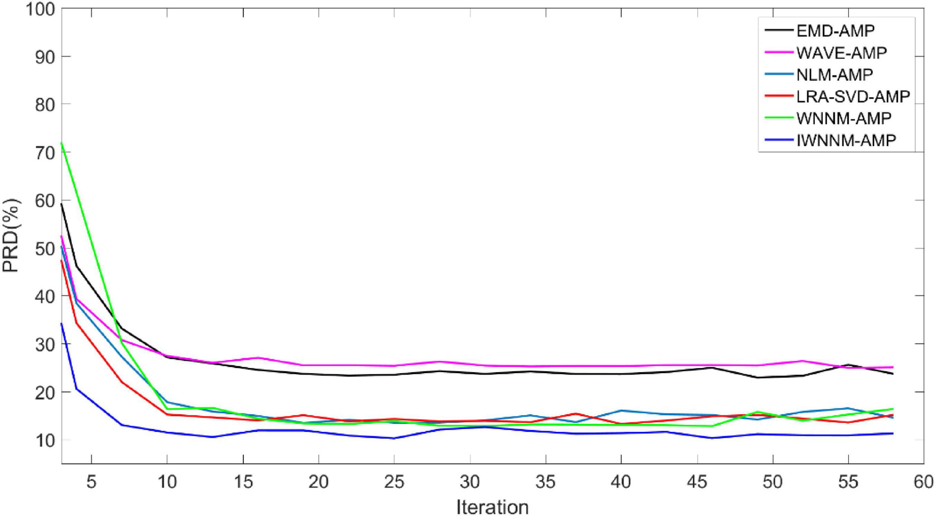
Figure 2. Comparison of PRD values with iteration numbers for six reconstruction algorithms under noise-free conditions.

The PRD value of the IWNNM-AMP algorithm is lower than that of the EMD-AMP, WAVE-AMP, WNNM-AMP, NLM-AMP and LRA-SVD-AMP algorithms, and the convergence speed is faster. After the number of iterations reaches 30, the PRD values obtained by the six algorithms change little. Therefore, this article will use the number of iterations K = 30 as an example to demonstrate the simulation results.

Figure 3 shows the curves of the PRD values of the six algorithms changing with the number of iterations when the measurement noise variance is 15 and the compression ratio CR = 5.12. In the presence of observation noise, all six algorithms have good convergence performance, and the reconstruction performance of the IWNNM-AMP algorithm is better than that of the other five methods.

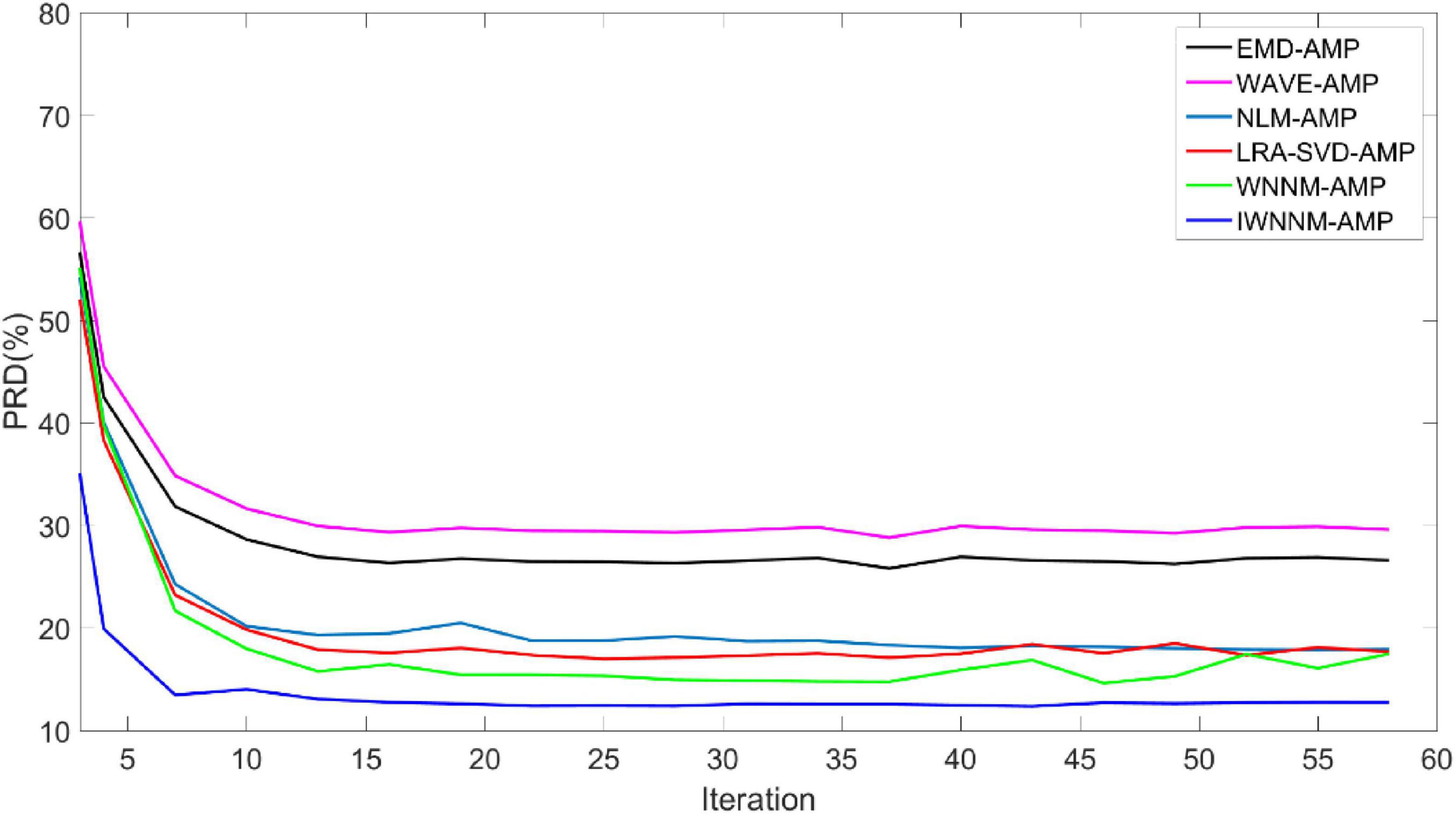
Figure 3. Comparison of PRD values with iteration numbers for six reconstruction algorithms under the condition of noise variance of 15.

4.3.2 The impact of different compression rates on reconstruction results

When the compression ratio varies from 1.03 to 5.12, the impact of the compression ratio CR on the performance of the six reconstruction algorithms is analyzed. Figure 4 shows the variation of PRD values of the six algorithms with compression rate when measurement noise is not considered and the number of iterations is 30. The experimental comparison results show that under different compression rates, the PRD value of the proposed method are generally the lowest, indicating that compared with other methods, the proposed method has better objective reconstruction performance. At the same time, as the CR value increases, the PRD of the reconstruction results of various methods gradually improves. Meanwhile, as the CR value increases, the PRD of the reconstruction results of the six algorithms gradually increases.

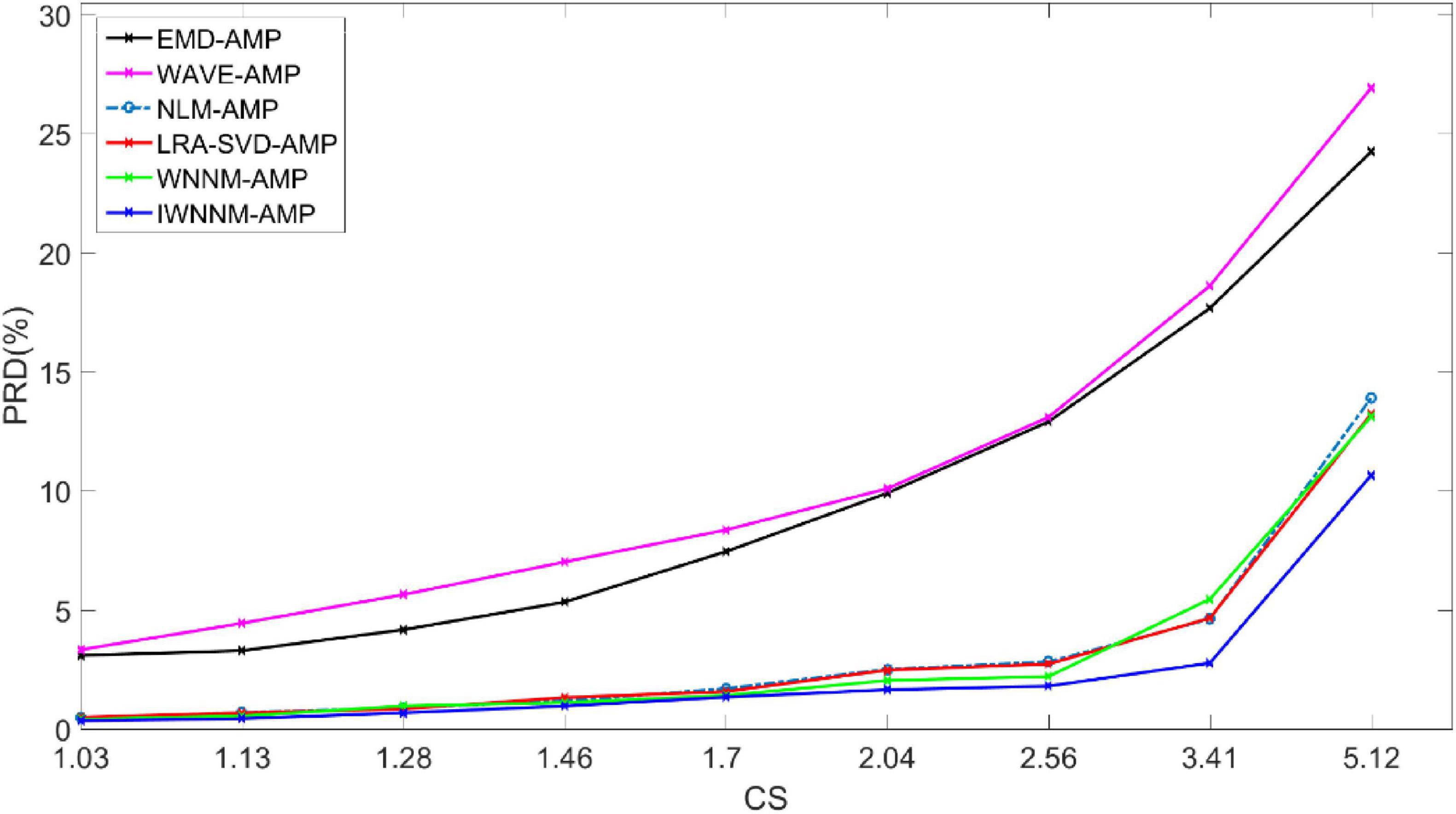
Figure 4. Comparison of PRD values with compression rate variation for six reconstruction algorithms under noise-free conditions.

When the CR is 1.7–2.04, the maximum PRD difference between the IWNNM-AMP algorithm and the EMD-AMP, WAVE-AMP, NLM-AMP, LRA-SVD-AMP and WNNM-AMP algorithms is 8.45. When the CR is 5.12, the IWNNM-AMP algorithm has the largest difference in PRD compared to the WAVE-AMP algorithm. The PRD of the proposed method is 13.59, 16.27, 3.24, 2.57, and 2.46 lower than that of the EMD-AMP, WAVE-AMP, NLM-AMP, LRA-SVD-AMP, and WNNM-AMP algorithms, respectively. As the CR value increases, the reconstruction performance of the IWNNM-AMP algorithm is better than that of the comparison algorithm.

Figure 5 shows the curve of PRD values versus compression ratio for six algorithms with a measurement noise variance of 15 and 30 iterations. In the presence of observation noise, the reconstruction performance of the IWNNM-AMP algorithm is better than that of the other five methods. At the same time, as the CR value increases, the reconstruction performance of the IWNNM-AMP algorithm is better than that of the comparison algorithms.

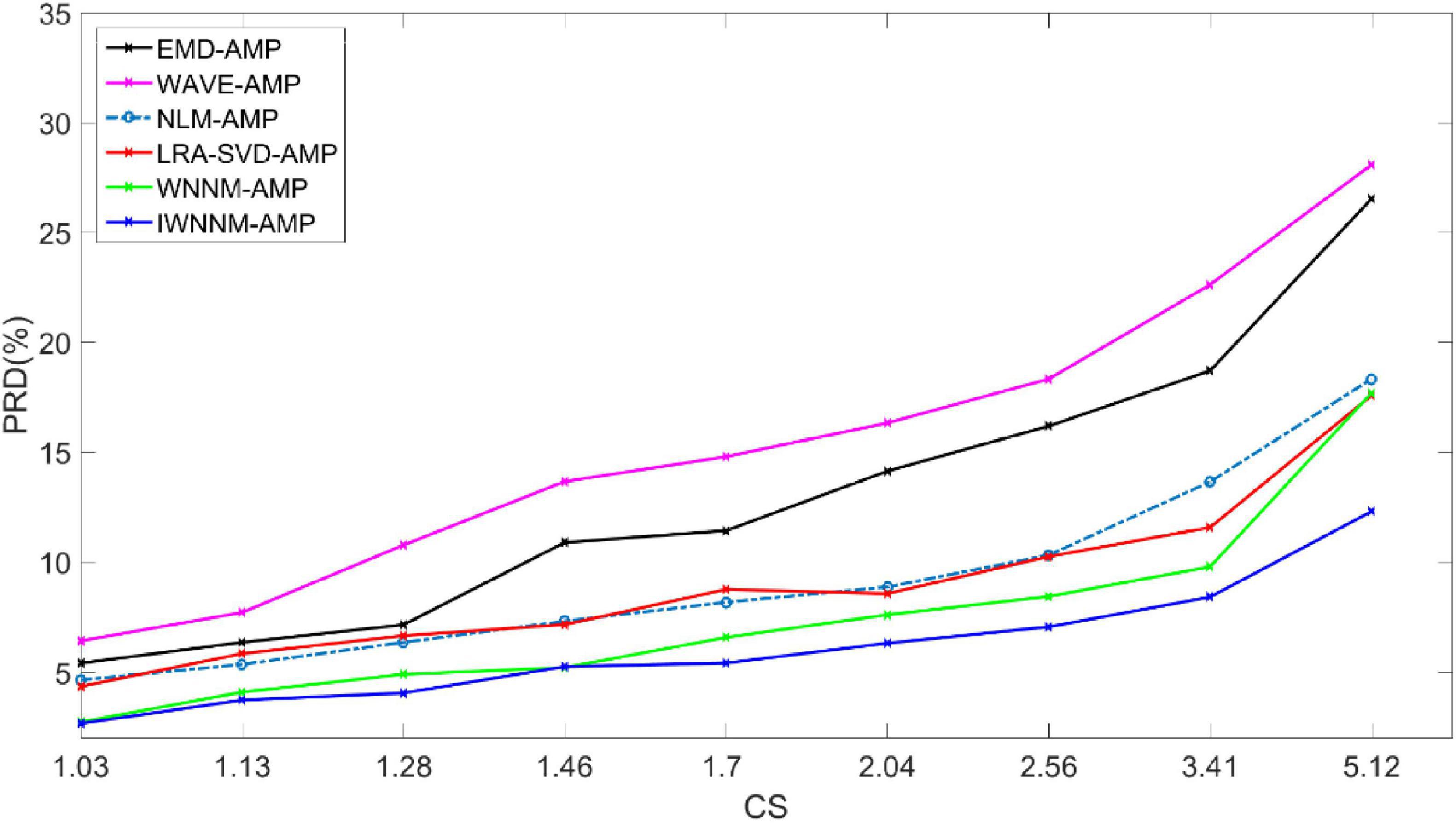
Figure 5. Comparison of PRD values with compression ratio for six reconstruction algorithms under the condition of noise variance of 15.

4.3.3 The impact of different noise levels on the reconstruction results

To verify the denoising effect of the algorithm under different noise levels, Gaussian white noise with noise intensities of 15 dB, 20 dB, and 25 dB was added to the 113th ECG signal, and the performance metrics of the six algorithms under different noise conditions were calculated.

Table 1 shows the average values of reconstructed PRD of the six algorithms under three different noise conditions when the compression ratio CR = 5.12 and the number of iterations is 30. The average experimental data show that when the noise variance is 15, compared with EMD-AMP, WAVE-AMP, NLM-AMP, LRA-SVD-AMP and WNNM-AMP, the PRD/RMSE values of the proposed method are lower than 14.296/0.044, 17.498/0.053, 6.389/0.014, 4.660/0.010 and 4.564/0.013, respectively. SNR/PSNR values were higher than 6.625/6.881, 7.605/7.605, 3.419/3.313, 2.741/2.778 and 2.704/2.706, respectively.

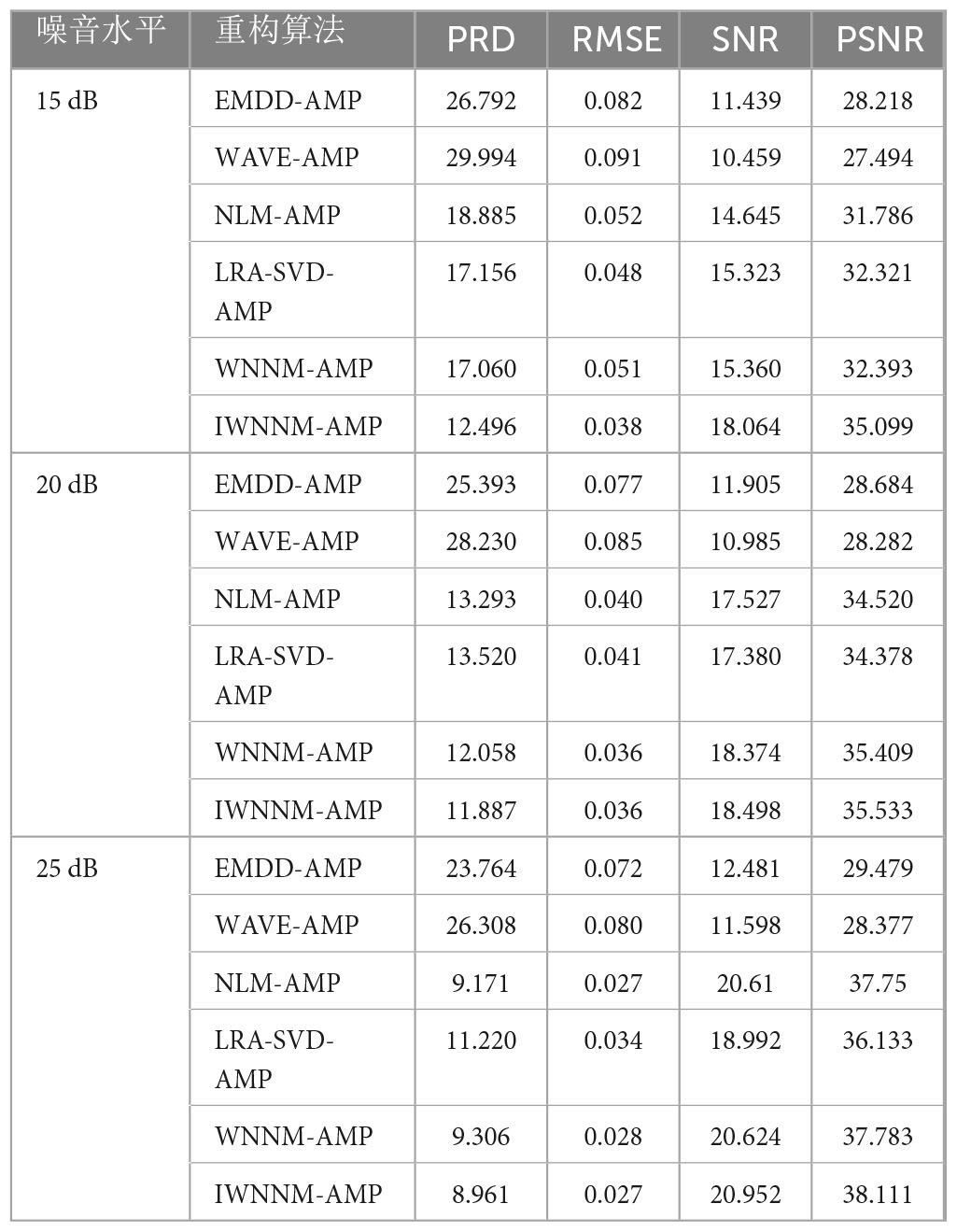
Table 1. Reconstruction performance of different algorithms under different noise.

The average experimental data show that when the noise variance is 20, compared with EMD-AMP, WAVE-AMP, NLM-AMP, LRA-SVD-AMP and WNNM-AMP, the PRD/RMSE values of the proposed method are lower than 13.506/0.041, 16.343/0.049, 1.406/0.004, 1.633/0.005 and 0.171/0, respectively. SNR/PSNR values were higher than 6.593/6.849, 7.513/7.251, 0.971/1.013, 1.118/1.155 and 0.124/0.124, respectively.

The average experimental data show that when the noise variance is 25, compared with EMD-AMP, WAVE-AMP, NLM-AMP, LRA-SVD-AMP and WNNM-AMP, the PRD/RMSE values of the proposed method are lower than 14.785/0.045, 17.347/0.053, 0.210/0, 2.259/0.007 and 0.345/0.001, respectively. SNR/PSNR values were higher than 8.471/8.632, 9.354/9.734, 0.342/0.361, 1.960/1.978 and 0.328/0.328, respectively.

The paired t-test method was used to statistically analyze the PRD values of different algorithms in Table 1, and P < 0.05 was considered to be statistically significant. t-tests were conducted on the PRD values of the IWNNM-AMP algorithm and other algorithms at different noise levels, and the results are shown in Table 2.

Table 2. t-test for PRD values of different algorithms.

From the results in Table 2, it can be seen that compared with the EMDD-AMP and WAVE-AMP algorithms, the reconstruction effect of the IWNNM-AMP algorithm is significantly improved (P < 0.001). This is because empirical mode decomposition and wavelet denoising require an understanding of the frequency domain characteristics of the signal, while the IWNNM-AMP algorithm is a blind denoising method that utilizes the structural features of the signal to achieve denoising, making it more advantageous in reconstructing compressed signals. Compared with the NLM-AMP algorithm, LRA-SVD-AMP algorithm, and WNNM-AMP algorithm, the IIWNNM-AMP algorithm has lower PRD values by 6.389, 4.66, and 4.56, respectively, when the noise variance is 15. However, when the noise variance is 20 and 25, the PRD values are relatively close (P > 0.05).

Figures 6–9 compare the reconstruction results of the IWNNM-AMP algorithm with three other algorithms from the subjective visual perspective under the condition of an additional measurement noise standard deviation of 20 and compression ratio CR = 5.12. Through the comparison of reconstruction results, we found that the NLM-AMP and LRA-SVD-AMP algorithms have poor reconstruction quality, indicating that these algorithms perform poorly in reconstructing measured values with noise. Compared to the WNNM-AMP algorithm, the IWNNM-AMP algorithm has better visual reconstruction effects and superior detail reconstruction capabilities.

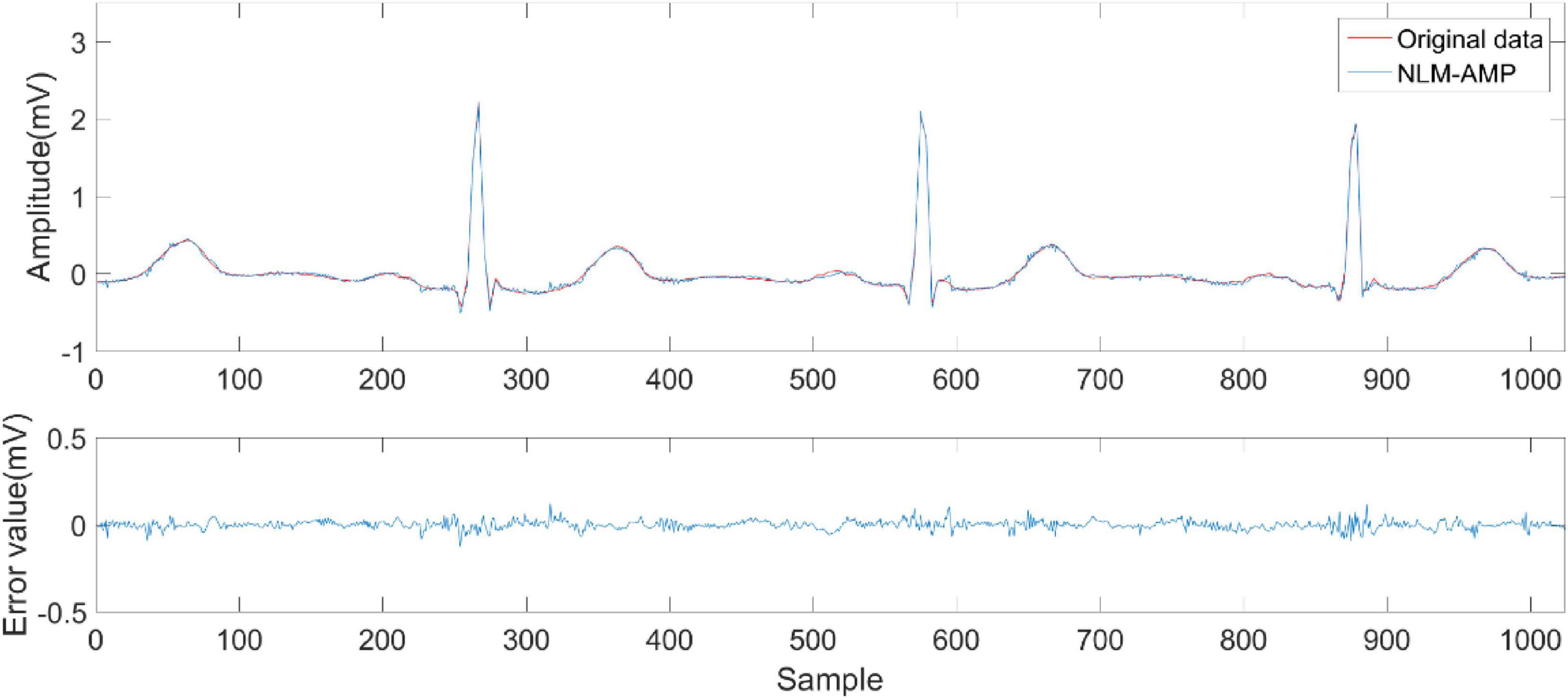
Figure 6. Reconstruction results of NLM-AMP algorithm.

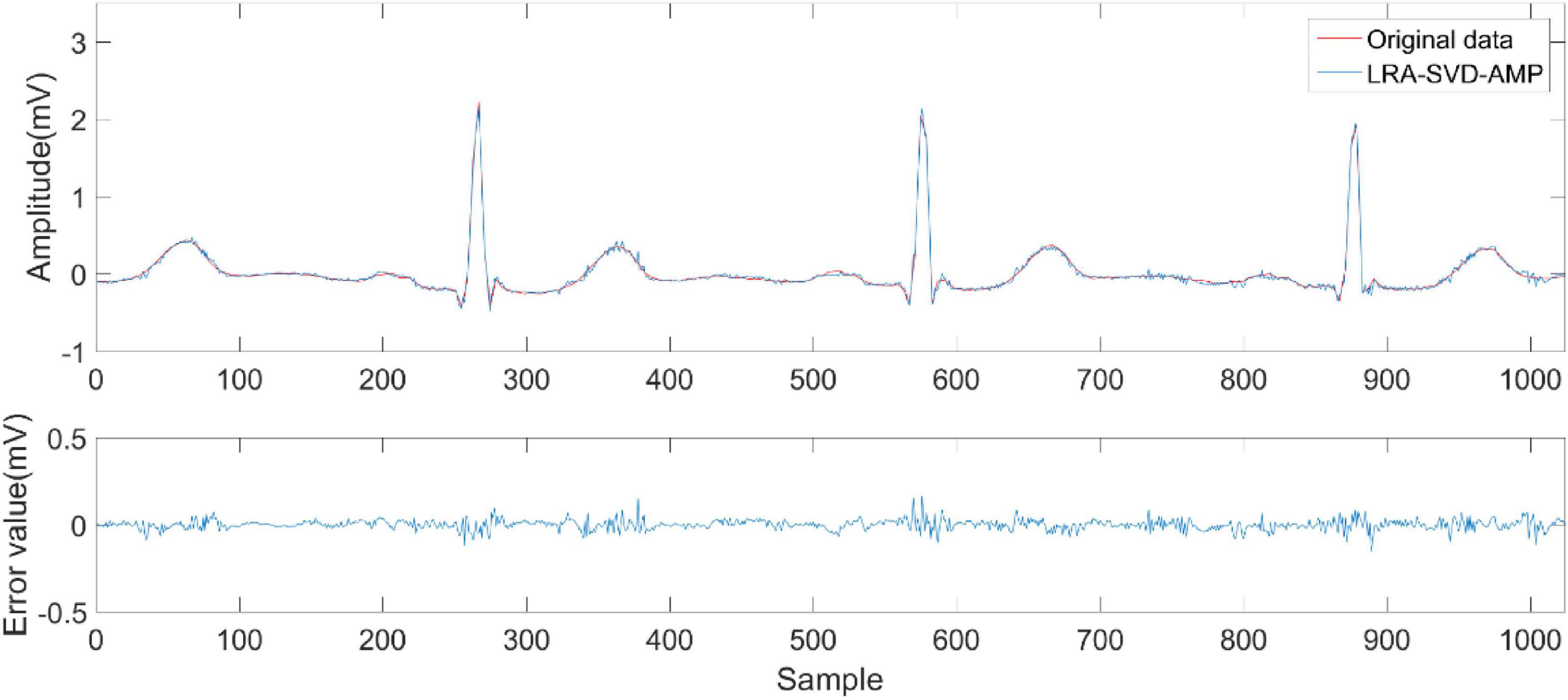
Figure 7. Reconstruction results of LRA-SVD-AMP algorithm.

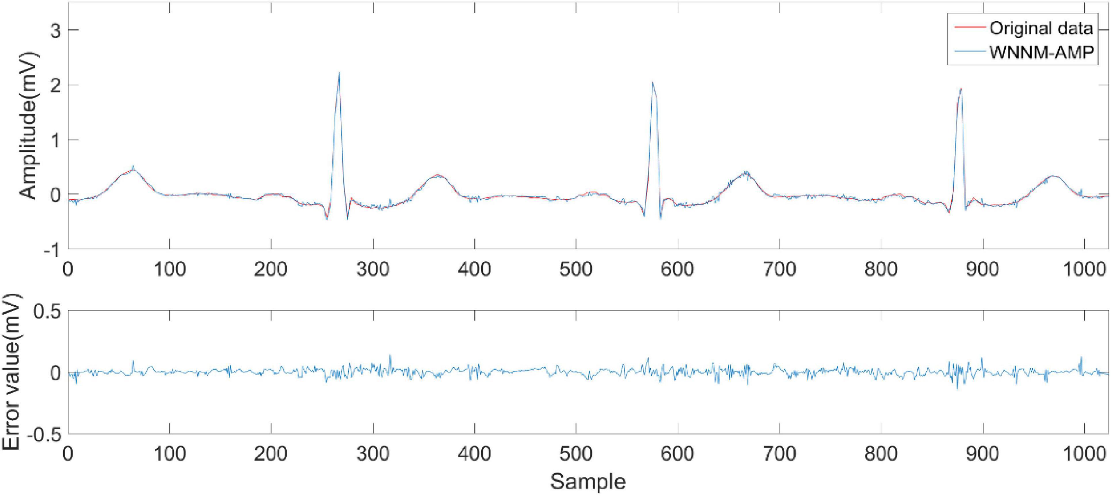
Figure 8. Reconstruction results of WNNM-AMP algorithm.

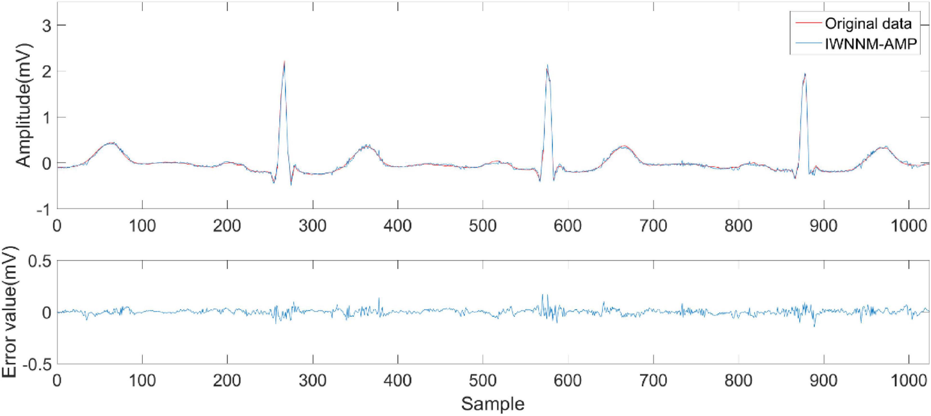
Figure 9. Reconstruction results of IWNNM-AMP algorithm.

4.3.4 Complexity analysis

Assuming the noisy signal x ∈ RN and the signal block qi ∈ Rd, the time complexity of calculating all similar blocks is o((N − d + 1)2). Considering that the time complexity is too large, the algorithm defines a window range wSize for signal block qi and calculates the similarity between signal block qi and the signal blocks within window range wSize. This not only reduces the time complexity, but also because similar blocks to a signal block are usually located around this signal block. Perform