
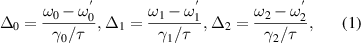
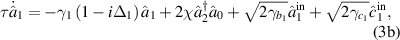
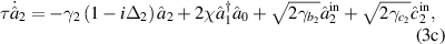
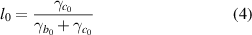
Remember me
Continuous variable multipartite entanglement is an important resource in quantum optics and quantum information. Non-degenerate optical parametric oscillator (NOPO), generally working in a resonant regime, can generate high quality tripartite entanglement. However, the detuning in a real experiment is inevitable and sometimes necessary, for instance, in an optomechanical system. We calculate the tripartite entanglement from a detuned triply quasi-resonant NOPO. Unlike the previous literature using inseparability criterion, we use the positivity of partial transpose, a sufficient and necessary criterion, to characterize the tripartite entanglement with full inseparability generated from a detuned NOPO. We also consider the influence of the pump and signal/idler losses on the tripartite entanglement. The results show that, the tripartite entanglement could exist even with a large detuning of several times cavity linewidth, and may be better for a detuned regime than for the resonant one under some conditions. With a fixed non-zero loss which always exists in a real experiment, an appropriate value of non-zero detuning could lead to the best entanglement. What's more, unlike the bipartite entanglement, which exists both below and above threshold, the tripartite entanglement only occurs for a nonzero classical amplitude of signal/idler field. The jumping between the tripartite and bipartite entanglement could make the NOPO become a quantum state switch element, which promises a potential application on the multiparty quantum secret sharing.
Continuous variable (CV) entanglement is an important quantum resource in quantum communication, quantum computation and quantum precision measurement [1–3]. Especially, the multipartite entanglement, is the core to realize quantum computation and quantum network. Tripartite entanglement, with the least number of entangled multi-party, is of great significance. Tripartite entanglement can be generated by coupling squeezed beams on beam splitters [4], or directly through nonlinear processes such as optical parametric down-conversion [5–9], second harmonic generation [10–13] and atomic four-wave mixing [14, 15]. Unlike method with beam splitter mixing of the same-frequency modes, direct optical parametric oscillator (OPO) could generate multicolor multipartite entanglement, which has wider applications into quantum internet [16–18]. OPO proves to be an effective device to generate high-quality entanglement because of its low loss and strong nonlinearity. Three-color tripartite (pump-signal-idler) entanglement can be directly generated by a nondegenerate OPO (NOPO) above threshold [5, 6]. Quadripartite Greenberger–Horne–Zeilinger (GHZ) entanglement [19] or cluster entanglement [20] were also experimentally realized in virtue of the spatial modes.
The OPO usually works in a resonant regime. The frequencies of signal/idler/pump fields are the same to the cavity frequency. The detuning is introduced if the frequency of at least one laser beam is not resonant in the cavity. The detuning should be avoided in a conventional experiment for entanglement generation due to its losses. However, the detuning is inevitable in a real experiment limited by the control precision of the cavity length. What's more, the detuning is required in some particular experiments. For a laser interferometer gravitational wave detector (GWD), the detuning of the signal recycling cavity greatly enhances the sensitivity at the optical spring frequency band [21, 22]. Adding an optical parametric amplifier further enhances the optical spring effect [23–25]. Recently, a detuned OPO is used to generate frequency-dependent squeezing which is required to achieve the GWD sensitivity beyond the standard quantum limit across the whole frequency band [26]. In the cavity optomechanics, the detuning is a feasible experimental parameter to control the optomechanical coupling strength [27–29].
The detuned OPO has been investigated in the literature [26, 30]. In the early days, people may focus its classical properties such as bistable or self-pulsing behaviour, which exhibits period doubling and chaos [31, 32]. Then the impact of detunings on the squeezing [33, 34] and bipartite entanglement [35] was reported. In recent years, multipartite entanglement from a detuned OPO is also reported. The tripartite entanglement remains with a large detuning [36]. The detuning of the signal field impacts tripartite entanglement more than that of pump field [37]. All of the above literature use the inseparability criterion to characterize tripartite entanglement. And few of them focus on the hysteresis properties of tripartite entanglement induced by the detunings in an NOPO.
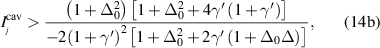
In this article, we consider all of the detunings, say that of the signal, idler and pump fields of a triply quasi-resonant NOPO. The positivity of partial transpose (PPT) [38, 39], instead of the inseparability criterion [4] is used to characterize the full tripartite entanglement. PPT is a sufficient and necessary condition to verify multipartite entanglement for  partitions, rather than the only-sufficient inseparability criterion. The results show that, although the tripartite entanglement generally decreases with the detunings increasing, it still exists with large detunings. Under some conditions, the tripartite entanglement may be better for a detuned regime than the resonant regime. Unlike the bipartite entanglement from NOPO may exist both below and above threshold, the tripartite entanglement only occurs with a non-zero solution of down-converted classical amplitude. This is reasonable because it is the pump depletion which constructs the quantum correlation between the pump and down-converted fields and finally leads to tripartite entanglement. We also consider the influence of the losses of the pump field and signal/idler field. Without detunings, the tripartite entanglement deteriorates with increasing loss. However, with detunings, the best entanglement may occur with a nonzero loss, even with a large loss. Furthermore, the tripartite entanglement exhibits hysteresis property like the classical field acts. By adjusting the detunings and the pump amplitude, the NOPO could be regarded as a quantum state (more precisely tripartite entangled state) switch.
The paper is organized as follows. Section 2 gives the Langevin equation and its steady-state solution. Section 3 gives the quantum Langevin equation and its solution in the Fourier frequency. A brief introduction of criteria of tripartite entanglement for inseparability and PPT is given in section 4. The numerical simulation of tripartite entanglement with/without detunings is given in section 5. The loss effect on the entanglement is simulated in section 6. In the discussion of section 7, the quantum state control with detuned NOPO is discussed.
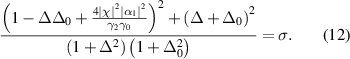
We consider the theoretical model of type-II NOPO shown in figure 1. A second order nonlinear crystal with the nonlinear coefficient of  is placed in a triangle cavity. The input pump field of a frequency ω0 is down-converted into two fields of frequencies ω1 and ω2. The γi
(
is placed in a triangle cavity. The input pump field of a frequency ω0 is down-converted into two fields of frequencies ω1 and ω2. The γi
( ) are the total loss parameters respectively of the pump, signal and idler fields. We consider the triply quasi-resonant case and define the detuning parameter as
where  are the resonant frequencies respectively corresponding to the pump, signal and idler fields, τ the cavity round-trip time. Neglecting all of the intracavity losses, the loss parameters are related to the amplitude reflection (transmission) coefficients ri (ti) of the coupling mirrors through

where  are the one-pass loss parameters corresponding to the input-output mirrors.
Figure 1. The theoretical model of non-degenerate optical parametric oscillator.  (
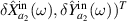
( ) are the annihilation operators of the incoming pump and signal fields, and
  (
( ) the corresponding output fields.
Download figure:
Standard image High-resolution imageThe Langevin motional equations, which could be derived from the Heisenberg motional equations, considering intracavity losses, are given by

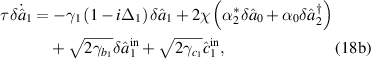
where  are the corresponding intracavity annihilation operators, χ the nonlinear coupling coefficient,
  the intracavity losses due to the absorption, surface scattering, and the total loss parameters
  . The
. The  are the annihilation operators of input fields. The
  are the annihilation operators of input vacuum fields from intracavity losses. For the convenience of numerical simulation, assuming
  ,
,  , we define the intracavity losses of pump and signal (idler) fields as
and
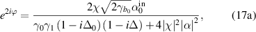
Using the semiclassical approach, we have  , where αi
and
, where αi
and  are the classical amplitudes and quantum fluctuations associated with the intracavity fields. Ignoring all of the fluctuations and intracavity losses, the equations of motion of the classical amplitudes are given by [33, 35]


The equations above could give the dynamical behavior of the cavity fields. However, to investigate the squeezing or entanglement generation, we focus on the steady-state results. Making the left side of the equation (6) be zero, the steady-state equations are given by [40]


Below the threshold, the gain of the down-converted fields is smaller than the loss, then the average amplitudes of the intracavity signal and idler fields are both zero, thus the steady-state solutions below threshold are given by
Above the threshold, the oscillation condition of triply resonant OPO requires the two detunings of down-converted fields are the same [40]

Solving equations (7), by multiplying the conjugate of the second by the third one, the pump threshold is given by
We can see that the pump threshold increases not only with losses (including intracavity and output coupling losses of all the fields) increasing, but also with the detunings Δ and Δ0 increasing. Then the pump parameter normalized to the pump threshold is given by
Note that we normalize the pump intensity to the real pump threshold including the detunings, unlike [40] where the pump is normalized to the resonant threshold. This normalization makes it convenient to study the variation of entanglement with the pump intensity with the detunings.
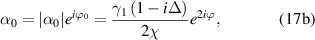
Using equation (7), we yield an equation of intracavity signal field
Two cases are related to the solution of equation (12) as follows.
Case 1: 
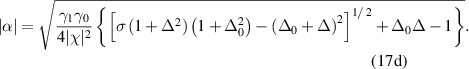
When  , the intracavity signal/idler intensity,
 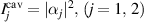 , has one nonzero solution
where  . The OPO operates in a monostable regime, shown in figure 2(a). However, the solution will not be stable if two conditions as follows are simultaneously satisfied [32, 33],
Figure 2. The normalized signal field intensity  vs the normalized pump parameter σ: (a) monostable curves, where
  ; (b) bistable curves, where
  . The blue solid lines denote stable solutions, the red dashed lines denote unstable solutions; (c) Region map of stability in the
  plane with
  denoted by monostable, bistable and unstable, respectively.
Download figure:
Standard image High-resolution image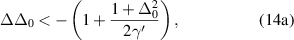
where we assume the two loss parameters of down-converted fields are the same, i.e.  for most cases in the following,
  . This unstable region is plotted with dashed line in figure 2(a).
Case 2: 
When 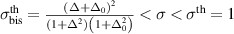 , three solutions are obtained, while only two of them are stable, so OPO may operate in a bistable regime, shown in figure 2(b). The
  is the bistable pump threshold. In this region, the two stable solutions of intracavity signal/idler intensity are given by


Above threshold, σ > 1, the solutions are the same to equation (15a ) and also to equation (13).
As analyzed above, OPO could operate in three regime, depending on the value of two detunings, Δ and Δ0. In figure 2(c), the three regime is shown in the  plane.
Now we consider the phases of intracavity average fields. Beginning with equations (7), and assuming the phases of intracavity pump, signal and idler fields are respectively  , i.e.
  ,
,  ,
,  , then the steady-state equations become


Assuming two down-converted fields have the same phase and the same intensity, i.e.  and
and  , then the steady-state solution above threshold in the monostable regime is given by

In the bistable regime, the nonzero steady-state solution is the same to that of monostable one, i.e. equations (17). This solution will be used in the following entanglement analysis.
Using the semiclassical approaches and only considering the quantum fluctuation operators of equations (3), the quantum Langevin equations are given by
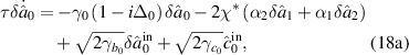
Introducing the quadrature amplitude and phase operators  and
and  , we can write equations (18) in the matrix form as

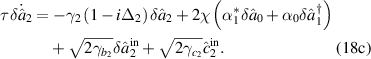
where  is the transpose of the vector associated to the quadrature operators. The drift matrix A is written as
where  and
and  respectively denote the real and imaginary part of the complex amplitude of the fields. For simplicity, the χ is assumed to be real, i.e. the phase-matching condition is fulfilled [40]. The diffusion matrix is given by
with two coefficient-related diagonal matrices
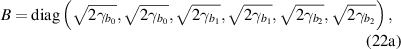
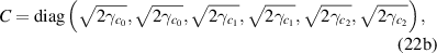
and  ,
,  are respectively the input vectors of vacuum fluctuations through the coupling mirrors and the intracavity losses.
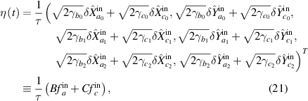
By Fourier transform of equation (19) with  and using equation (21), we have

where  and
and  are respectively the Fourier transform of f(t) and
  ,
, 
 , and
, and  has a similar form with
  . Using the input–output relation of the cavity of
  [41], we have

with 
 .
.
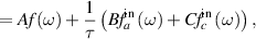
Solving equations (23) and (24), we have
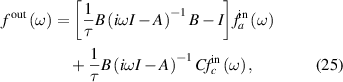
where I is the identity matrix. For convenience, the analyzing frequency normalized to the linewidth of the fundamental mode,
Comments (0)