1 Introduction

The human brain consists of around 80 billion neurons of different shapes and sizes. These neurons are highly interconnected and form complex networks in the brain with information exchanged between neurons through chemical and electrical synapses (Ioannides, 2006). The electrical activity of a single neuron is too small to be detected from outside the brain. The well-known non-invasive signals of electroencephalography (EEG) and magnetoencephalography (MEG), are the result of synergistic accumulation of contributions from a huge number of activated neurons (Hämäläinen et al., 1993; Lopes da Silva, 2013; Singh, 2014). EEG and MEG are members of the wider family of neuroimaging techniques capable of mapping mass regional activity from the brain (Horwitz et al., 2000; Bandettini, 2009; He et al., 2011). These techniques can identify activity confined to a small enough region that belong to specific cytoarchitectonic areas in the cortex (Moradi et al., 2003) or specific nuclei (Papadelis et al., 2011, 2012). It is universally acknowledged that what distinguishes EEG and MEG from other neuroimaging techniques is their high temporal resolution which is in the order of a millisecond or less (Hämäläinen et al., 1993; He et al., 2011; Lopes da Silva, 2013; Baillet, 2017; Michel and He, 2019).

EEG measures the electric potential difference between the ground and other scalp surface electrodes. In the case of MEG, the instantaneous changes in the magnetic field are measured using either single coil sensors (magnetometers) or differential combination of coils (gradiometers) (Hämäläinen et al., 1993; Singh, 2014). Modern instruments provide a collection of sensors for each modality arranged uniformly to cover as much as possible the surface of the head around the brain (Baillet, 2017).

The standard way to estimate the activity inside the brain is through source reconstruction algorithms (Asadzadeh et al., 2020), which transform the timecourses of sensor recordings (signal space description) to timecourses of few or many generators in the brain (source space description) (Ioannides et al., 1990; Mosher et al., 1999; Michel and Brunet, 2019). Source reconstruction using EEG and/or MEG, demands making a model which is based on assumptions some explicit while other implicit; a model allows computations to be made for the contribution from any assumed source configuration (forward problem) and hence through applications of different methods (which also contain assumptions) a best fit solution can be determined (Scherg, 1992; Mosher et al., 1999; Michel and Brunet, 2019; Asadzadeh et al., 2020). For EEG, a complex model is necessary to take into account the high resistivity of the skull (Michel and Brunet, 2019) and the changes in conductivity between different tissues that distort the electric current (Baillet, 2017). In contrast, for MEG, a simpler model is sufficient as the propagation of the magnetic field is not greatly affected by the conductivity details (Hämäläinen et al., 1993; Lopes da Silva, 2013; Singh, 2014). Nevertheless, in both cases, the accuracy and spatial resolution depend heavily on the accurate co-registration of the sensor's position to the head (Akalin Acar and Makeig, 2013; Michel and Brunet, 2019).

There are numerous EEG/MEG studies involving animals and human subjects that aim to understand the underlying mechanisms of different sensory systems, by using different kinds of external stimulation. To understand the processing mechanisms of any sensory system, apart from identifying the location of the brain areas involved in the processing, what is also necessary is the study of the communication between those areas (He et al., 2011). During an experiment, a large number of identical stimuli are presented to the subject, with each presentation referred to as a single-trial (ST). Even though identical stimuli are used, each stimulus evokes a response that could vary considerably between trials (ST variability), in terms of the timing and topography of the EEG and MEG signal (Liu et al., 1998; Ioannides et al., 2002; Stephani et al., 2020). The interest in ST variability of EEG and MEG sensory evoked responses was raised when variability of ST responses was also demonstrated with functional magnetic resonance imaging fMRI (Duann et al., 2002). However, we will not discuss the fMRI ST variability further because the timescales involved (few seconds) are more than two orders of magnitude larger than the timescales relevant to the variability of the EEG/MEG responses (a few milliseconds).

In this paper, we utilize simultaneous EEG-MEG recordings elicited by somatosensory electrical stimulation to address the following objectives. The first objective of this study is to extract the activity of specific brain generators at particular time-points relative to the stimulus onset, while avoiding the assumptions typically associated with source reconstruction techniques. This is accomplished using Virtual Sensors (VS), which are created through linear combination of different channels. We demonstrate that such a VS can effectively capture the activity generated by generators for each ST. Combining this capability with knowledge about the location and timing of well-known generators, yields a data-driven estimate of the ST timecourse of these specific, well-known cortical and subcortical brain regions. The second objective is to verify whether or not accurate estimates of cortical and subcortical generators can indeed be extracted for each ST. The third objective of our study is to explore the usefulness of having simultaneous measurements of EEG and MEG, which are known to be derived from complementary mathematical properties of the common current density vector generated by neural electrical activity. The fourth objective is to explore the variability of the ST activations derived from the VS by utilizing clustering techniques. The fifth objective is to compute the connectivity across the ensemble of all STs using a linear and nonlinear connectivity metrics and compare the results with current literature. The sixth and final objective is to explore the variability in connectivity across STs in general and to investigate the distinct types of connectivity that prevail in the different sets of STs that clustering methods have identified.

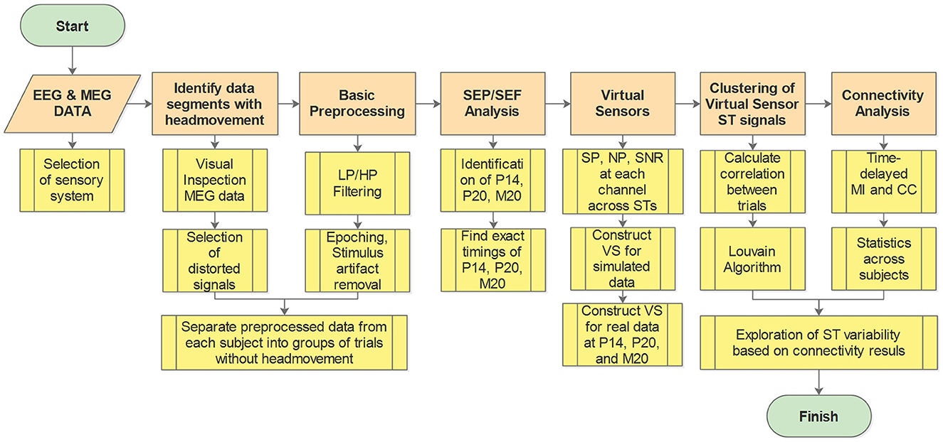
2 Materials and methods

The workflow diagram illustrating the methodology is presented in Figure 1. In the Figure, the main analysis steps are depicted in orange, while the submethods for each step are shown in yellow. A key preliminary task was to decide which sensory system to study and how this system will be stimulated. Having in mind the objectives of the study, we eventually chose to work with brain responses to somatosensory stimulation for reasons explained in Section 2.1. After this preliminary task was completed and the data obtained (Section 2.2), the first step of the pipeline involved identifying and excluding data segments contaminated with artifacts, e.g., caused by the subject's head movement during the recording (see Section 2.3). Preprocessing of the data was then conducted, which includes various filtering techniques and removal of stimulus artifacts (see Section 2.3). Subsequently, the Somatosensory Evoked Potentials (SEPs) and Fields (SEFs) were analyzed to identify the timings of the first evoked responses in the thalamus and the somatosensory cortex (see Section 2.4). Moving forward, VS were utilized to extract spatiotemporal estimations of activity in the thalamus and the primary somatosensory cortex S1 (see Section 2.5). Cluster analysis was then employed to identify and group spatiotemporal estimations with similar information (see Section 2.6). Next, the clustered data were utilized to estimate thalamocortical connectivity (see Section 2.7). Finally, the estimated connectivity values were further analyzed to differentiate the different types of influences between the thalamus and the cortex implied by the linear and non-linear connectivity measures (see Section 2.8).

Figure 1. Work flow diagram. Orange boxes show the main analysis steps while the yellow boxes give a brief description of the processing and analysis methods at each step. LP, low pass; HP, high pass; SEP, somatosensory evoked potential; SEF, somatosensory evoked fields; SP, signal power; NP, noise power; SNR, signal to noise ratio; ST, single trial; VS, virtual sensor; MI, mutual information; CC, correlation coefficient.

2.1 Selection of sensory system

The EEG and MEG neuroimaging modalities are usually used for the study of the somatomotor, visual and auditory systems in the brain. Any one of these three modalities could be used in our study; the selection was influenced by how well the primary requirements, which were to have good a priori information about the timing and location of the first evoked responses in the thalamus and the cortex. For each one of these three sensory modalities (somatosensory, visual and auditory), there is good evidence in the literature about the timings and precise location of the first arrival of the responses evoked by stimuli, first in the corresponding nucleus of the thalamus [ventral posterolateral (VPL) nucleus, Lateral Geniculate nucleus (LGN) and medial geniculate body (MGB)], and a few milliseconds later to the specific primary sensory cortex [S1; Broadman Area 3b (BA3b), V1; BA17 and A1; BA41;42].

There are also common drawbacks and problems specific for each sensory modality. The common feature (drawback) is that for each modality the response to each individual stimulus is different. As demonstrated in our earlier MEG studies, for stimuli well above the sensory threshold, but relatively weak to startle the subject, the early cortical response in the primary sensory cortex is so variable that little or no evidence of it can be traced for most STs in either somatosensory (Ioannides et al., 2002; Hu et al., 2011, 2014; Stephani et al., 2020; Waterstraat et al., 2021), visual (Duann et al., 2002; Laskaris et al., 2003, 2004; Bagshaw and Warbrick, 2007) or auditory (Liu et al., 1998; Kisley and Gerstein, 1999; Laskaris and Ioannides, 2001, 2002; Goldman et al., 2009) cortex. Analysis of the ST data at signal and source levels focusing on the cortical responses has demonstrated an individual statistical signature of the evoked response that was reproducible across days (Liu et al., 1998). Also, there is a clear influence of the prestimulus activity in the primary sensory cortex on the early evoked response in the same area for somatosensory, visual and auditory stimulation (Laskaris and Ioannides, 2002; Laskaris et al., 2003). Ideally, these problems of studying ST variability can be addressed by using strong stimuli and asking the subject to report on the perceived qualities of each ST stimulation. However, such an approach is impractical because it would require long recording times and it will be very tedious and uncomfortable for the subject. It is also important to note that what we call drawback and problem above are really properties of a healthy brain, so if we want to understand normal brain function we must accept and account for the observed variability in ST responses to identical stimuli.

There are also further problems specific to each sensory modality. For visual stimulation, the placement of a stimulus to a specific quadrant of the visual field allows for a precise definition of which part of V1 the activity should be seen on the left or right hemisphere and on the upper or lower side of the calcarine fissure, provided that the subject can fixate on a fixation stimulus. No fixation is needed for auditory stimuli, but the pathway from the ear to A1 is not strictly unilateral but bilateral: auditory stimulation of one ear exiting the thalamus and the A1 on the ipsilateral and contralateral hemisphere with the pathways crossing the hemispheres at multiple subcortical levels. In contrast, the cortical sources to somatosensory stimulation are well separated and away from the mid-line of each hemisphere (for stimuli delivered in the left and right upper limbs). In addition, the reporting by the subject of the qualities of perception of each stimulus is the only way of ensuring that the targeted pathway was activated in each ST. These limitations of the visual and auditory systems (for achieving the objectives of our study) prompted us to select a fairly strong hand stimulation, i.e., electrical stimulation of the median nerve of the wrist. This type of stimulation has its own problems which we describe next in the context of other choices for exciting the somatosensory system.

Pure somatosensory stimulation can be achieved with the use of tactile stimuli, which however are difficult to control precisely (e.g., keeping the level of pressure applied constant) and/or do not afford precise timing, e.g., using a balloon. An electrical stimulation with a short pulse (sub-millisecond duration), provides an easier way of achieving precise timing. Unfortunately, the nature of electrical stimulation introduces a strong artifact, which is smaller for weak stimuli and reduces further for foot (tibial nerve) than hand electrical stimulation. Foot stimulation however is close to the top of the central sulcus with left and right primary sensory areas close to each other. Considering all factors we settled on the use of somatosensory dataset (Antonakakis et al., 2019); hereafter we will refer to electrical median nerve stimulation of the wrist as Electric Wrist (EW) stimulation, for consistency with the earlier analysis of the same data by Antonakakis and colleagues. This set includes simultaneous EEG and MEG recordings for three subjects in response to over 1,000 STs of EW stimulation at the right wrist. The EW stimulation is strong enough to produce a small twitch of the thumb. This ensures that there is a visible response for each stimulus applied, without the need to ask for a report from the subject. On the cost side, there is an early artifact in the signal caused by the strong electrical stimulus and the inevitable involvement of the motor system. A compromise of the advantage and disadvantage of the choice of a strong EW stimulation is made in the way the artifact is reduced but not completely removed as can be seen in the Supplementary Figures S2, S3. The delivery of a large number of trials takes a rather long period of time (9 min) with a stimulus that is rather slightly annoying, so some small movement could be made. While for EEG the removal of STs close to each movement is sufficient (because the electrodes are fixed on the scalp) for MEG this implies that the initial coregistration of the MEG sensors with the head is lost after the first movement.

2.2 Data description

We used simultaneous EEG and MEG data, collected in response to somatosensory stimulation, from three right-handed healthy human subjects. The experiments for data collection were conducted at the Institute of Biomagnetism and Biosignal Analysis, Muenster, Germany. The EEG/MEG recordings were provided to us in an anonymized form by the corresponding author of the study (Antonakakis et al., 2019) and co-author of this paper. The EEG recording involved 74 EEG channels and six auxiliary channels for eye movement detection. For MEG recording, a whole-head MEG system with 275 axial gradiometers was utilized. Further details regarding the EEG/MEG systems can be found in Antonakakis et al. (2019). In that study, three different types of stimulation were employed: Pneumato-Tactile stimulation using a balloon diaphragm, Braille-Tactile stimulation, and Electrical-Wrist (EW) stimulation of the right median nerve. For the current study, we exclusively utilized data acquired in response to EW stimulation. The electrical pulses delivered to the wrist had a duration of 0.5 ms, and the stimulus intensity was adjusted to elicit observable thumb movement in the subject. The data was sampled at a frequency of 1,200 Hz, and an online low-pass filter of 300 Hz was applied. The experiment consisted of 1,198 trials (repetitions) with an inter-stimulus interval (ISI) ranging between 350–450 ms.

2.3 Data preprocessing

Prior to initiating any data preprocessing, we excluded recorded periods during which large artifacts were present which are likely to involve head or body movements or large scale muscle activity like teeth clenching. Head movement during recordings significantly distorts the signals, particularly the MEG signals. Given that the MEG sensors are stationary above the head, even a small head movement causes large signal distortions across the entire sensor array that can be easily identified by visual inspection of the raw signals. Therefore, to ensure that the signals used in our analysis pipeline were free from movement artifacts, we employed a simple method to identify and exclude the trials associated with head movement. The raw signals from all MEG channels were plotted in a single plot, with each channel displayed consecutively (refer to Supplementary Figure S1). Visual inspection of the raw signals throughout the entire recording duration identified periods exhibiting significant signal distortions across all channels. These periods, along with a 1 s buffer before and after the identified noisy segments, were marked for exclusion. The STs in each period between the cut-out segments were identified as distinct set of trials, for which there was no pronounced distortion observed across all channels and hence no large head (or body) movement. This is a conservative approach because, it eliminates not only movement artifacts but also any other influence that is felt across the MEG sensor array; this conservative segmentation of the data was performed for all three subjects.

Moving to the preprocessing of the selected data, the first step was the reduction of the artifact created by the electrical stimulation, from both the EEG and MEG raw signals. For the reduction of the stimulus artifact, a segment from the background data in the pre-stimulus period (−18.3 to −5 ms) together with a segment of data containing the stimulus artifact (−5 to 8.3 ms) were multiplied by a Generalized Logistic function and combined to replace the stimulus artifact period. Detailed description of the stimulus artifact reduction method can be found in the schematic diagram shown in Supplementary Figure S2. As a second step, the EEG and MEG data were high-pass filtered at 1 Hz, and any noisy channels were removed. In the case of EEG, the mean of all channels was used to re-reference the signals of individual EEG electrodes. Furthermore, notch filtering at 50 Hz and its harmonics (100, 150, 200, 250 Hz) was applied to remove power line noise in the EEG and MEG signals. Next, the data were band pass filtered in the frequency range (20, 250 Hz). Once the data were cleaned and filtered, they were parsed into epochs (trials) of 0.3 s in total duration. Each trial consisted of signals starting 100 ms before (pre-stimulus period) and 200 ms after (post-stimulus period) stimulus onset. Subsequently, the identified trials with large movement were excluded and the remaining trials were separated into groups of trials free of movement artifacts. Finally, for each subject, the three groups with the highest number of trials were selected for further analysis. The number of trials in each group and the selected group of trials are shown for each of the three subjects in the Supplementary Table S1. This overcautious approach ensures that in each one of the groups separated out the head was in the same position for all the trials in each group.

2.4 Somatosensory evoked potentials/fields

While the EW stimulation excites many areas across the brain, both invasive and non-invasive experiments with humans have identified the time of the first arrival of the signal in the area of the thalamus at around 14–16 ms post-stimulus onset (Buchner et al., 1995; Hanajima, 2004; Porcaro et al., 2008; Götz et al., 2014; Politof et al., 2021). Then, the signal travels in a dorso-lateral direction reaching the primary somatosensory cortex (S1) at around 20 ms post-stimulus onset (Allison et al., 1991; Peterson et al., 1995; Gobbelé et al., 1999; Porcaro et al., 2008; Politof et al., 2019, 2021). For our purposes, what is important is that these are the first arrivals of the evoked response at the level of the thalamus and the cortex and they are therefore the signal components least influenced by activity in the many other cortical areas that come later. These somatosensory responses can be easily identified in the signal space as prominent peaks by calculating and visualizing the so-called Somatosensory Evoked Potentials (SEPs) and Fields (SEFs), from the EEG and MEG data, respectively.

For the visualization of the SEPs and SEFs, we first calculate the average across the ST timecourses of all the EEG chanels and MEG channels, respectively. Then the average of the EEG (SEPs) and MEG channels (SEFs) is plotted separately for the time window 50 ms prior and 100 ms post-stimulus onset. In the same Figure, we also show the topographies of the averaged EEG and MEG data at the identified prominent peaks in the SEPs and SEFs. This is done for each subject and for each of the three groups of trials. Knowledge of the location of the thalamic and cortical generators and the physics of their electrical activity predict which components will be seen best with EEG and/or MEG. Previous studies align well with these expectations. Specifically, it is expected to find the (EEG) components P14, (P/N20), (N/P30) and (P/N40) in the SEPs (Politof et al., 2019). The labels P and N refer to the polarity of the peak (positive, negative) but note that for tangential superficial sources the P/N for EEG will appear in different electrodes. The number in the labeling of components corresponds to the peak latency. These cortical activations are expected to appear in the (MEG) components M20, M30, and M40 of the SEFs, i.e., the EEG and MEG are expected to “capture” the activity of the cortical generators that become active at 20, 30, and 40 ms (Kakigi, 1994; Papadelis et al., 2011; Politof et al., 2019). In contrast, no prominent M14 component (the SEF analog of the SEP P14) is expected because the location of the thalamus is close to the center of the head, which is bounded by the high resistivity and nearly spherical cranium; in such a geometry configuration the magnetic field outside the head, generated by electrical activity in the thalamus is almost zero, because the dominant direction of the electrical current dipole is in the silent radial direction (Kimura et al., 2008; Papadelis et al., 2012; Politof et al., 2021). In this study, we focus on the first early components at around 14 ms (P14) and 20 ms (P20, M20) since these are considered to be the first entries in the thalamus and the cortex, respectively.

2.5 Virtual sensors 2.5.1 Linear spatial filters applied to a composite model signal

We have adopted a data-driven definition of separate linear combinations of EEG and MEG channels to extract from the raw EEG and MEG signals the early timecourses of the brain activity at the level of the thalamus and Somatosensory cortex. The linear combinations of channels are defined at two times. First around 14–15 ms when the evoked activity reaches the VPL nucleus of the thalamus. The VPL is the end-point of the spinothalamic tract: it is the main gate for activity elicited by somatosensory stimuli to enter the thalamo-cortical circuit. Within a few ms, around 18–20 ms the evoked activity reaches the primary somatosensory cortex, Broadman Area 3b (BA3b). We will simply refer to the output of these two linear filters as the activity of the thalamus and cortex hereafter, providing further clarification wherever this is needed. We will first illustrate the logic behind the approach we have taken and justify the label as virtual sensor (VS) of our seemingly simplistic linear spatial filter we have designed. The approach is illustrated using a simple, yet realistic scenario, which approximates reasonably well the findings of many earlier studies of the variability of responses to somatosensory stimuli (Ioannides et al., 2002; Stephani et al., 2020). We know that the EW stimulation elicits the first evoked responses at the level of the thalamus at the VPL around 14–15 ms and few ms later the evoked response can be identified at the cortical level in the Broadman Area (3b). Each of these responses is a focal well-circumscribed activation that can be approximated well by a single equivalent current dipole (ECD).

We generate a model signal, for the system we wish to study, which we will refer to hereafter as the composite model signal (CMS) to contrast it with the actual measurements which we will refer to as the measured response to EW (MRtEW). The CMS is a mixture of a computer-generated signal (sum of two ECDs, one for the thalamus and the other from the cortex) to which we add realistic background brain activity from a segment of the pre-stimulus period of the MRtEW. The CMS for each ST is the sum of two computer generated signals and a segment of pre-stimulus period of that trial (from −70 to −20 ms with respect to the onset of EW stimulus at 0 ms), from the actual background of the preprocessed EEG and MEG data. Each ECD of the CMS is modulated by a Gaussian function with fixed shape, full width of 5 ms at 5% of the maximum and strength adjusted so that the signal generated at the peak is comparable to the signal at the peaks of the MEG and EEG signal of single trials. A jitter is allowed in the latency of each ECD onset, by varying the latency of the center of the Gaussian form factor within a range of 4 ms, i.e., 2 ms on either side of the mean latency of 15 ms for the thalamic ECD and 20 ms for the cortical ECD. The random latency within the 4 ms range is varied independently for the thalamic and cortical ECDs. The location and direction of the ECD are fixed to what others have reported before for these two centers from EEG (Porcaro et al., 2008; Götz et al., 2014), MEG (Tesche, 1996) and MEG with fMRI (Papadelis et al., 2012) studies. The forward problem computation employed a head model constructed using a realistic three-layer (brain, skull, scalp) Boundary Element Method (BEM) volume conduction model of the head, based on a template MRI fitted to the electrode montage used for subject 1. The EEG and MEG signals were computed at the same locations as were given for the MRtEW experiment: 71 electrodes on the scalp for the EEG and 271 locations of the radial gradiometers inside the dewar, for the MEG sensors. The EEG- and MEG- CMS signals for one random ST are presented in the plots A and C of the Supplementary Figure S4, respectively. Plots C and D of the Supplementary Figure S4, show EEG and MEG topographies, respectively, for different time points at and around the peak latencies of the input ECD signals, illustrating the emerging distinct patterns (as expected from physics) at the ECD's peak latencies for that ST (e.g., 15 and 20 ms)

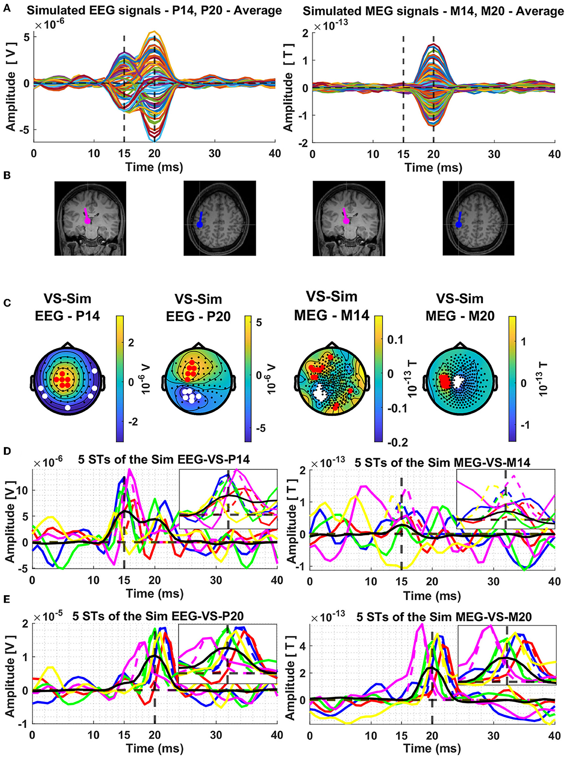
The next display, Figure 2, shows results for the average signal. The resulting butterfly plots for the average signals are displayed in row A of Figure 2, on the left half for the EEG and on the right half for the MEG. The dipole locations are shown in the next row (B) of the Figure 2 and in the third row (C) the topographies at the peaks of the thalamic and cortical ECD activations, which correspond exactly with the extrema of the butterfly plots shown in row A of Figure 2.

Figure 2. Average composite model signals (CMS) and source reconstruction of the modeled thalamic and cortical equivalent current dipoles (ECD) using the Virtual Sensor (VS) method. The average CMS signals across the 239 trials are shown in Panel (A), for EEG and MEG, in left and right columns, respectively. Panel (B) depicts the location and orientation of the ECDs plotted on the template coronal MR image for the thalamic dipole and axial MR image for the cortical dipole. Constructed Virtual Sensors are shown in Panel (C), with red colors indicating the selected sensors with positive and white color the sensors with negative amplitude. The VS extracted activations of the ECD in the thalamus [Panel (D)] and in the cortex [Panel (E)], using the EEG (left column) and MEG (right column) generated data are shown for five random Single Trials. In all four plots shown in Panel (D, E), the same five colors are used to differentiate between the VS signals of each ST, black solid lines show the average of all the 239 trials and the dashed vertical lines indicate the mean time of the peak activity of the input ECD signals across all the trials. The box in the top right quadrant of each plot of Panels (D, E) features zoom versions in the period 10–20 ms and 15–25 ms for the thalamic and cortical VS, respectively.

In left half of Figure 2B, the two displays show the thalamic ECD in a coronal MRI slice (at the level of VPL) and the cortical ECD in a fairly superficial axial MRI at the level of BA3b; The anatomy in Figure 2B is placed under the EEG butterfly plot (Figure 2A). Each EEG topography (Figure 2C) is placed directly below the ECD responsible for the corresponding peak latency. In the right half of Figure 2B, the display of the two ECDs is repeated again for the corresponding MEG butterfly (right half of Figure 2A) and topographies (right half of Figure 2C).

The MEG activity generated by the nearly radial thalamic ECD is much weaker, with a ratio of 10:1, compared to that generated by the nearly tangential cortical ECD. As a result, only a slight swelling but no clear peak is seen at the latencies of peak thalamic activity. A clear and nearly symmetric dipolar pattern is seen in the topography of the MEG signal at the latency of the peak of the cortical dipole, which is rotated by 90 degrees relative to the pattern of the EEG at the same latency. These patterns are as expected from physics, and they can be used to prescribe a completely data-driven and robust sensor-based analysis suitable for both average but also for ST signals. The procedure for designing such a robust spatial filter, will be described after we use the knowledge of the laws of physics to justify labeling these spatial filters “virtual sensors” for the underlying active sources.

2.5.2 Virtual sensor interpretation of our spatial filters

In EEG and MEG we are usually concerned with frequencies below 1 kHz, a range where active changes in the current density distribution in the brain are slow enough for the time derivatives to have negligible effect, i.e., for the quasistatic approximation of Maxwell's equations to be valid (Hämäläinen et al., 1993). In the quasistatic regime we can consider topographies of sets of MEG, EEG or even intra cortical EEG (icEEG) or intra cortical MEG (icMEG) as (nearly) equivalent representations of the current density changes that took place at that instant). Without any loss of generality we can assume that for each single trial we have the timecourses yj1(t) and yj2(t) for each of the two generators, respectively, that are scaling some normalized topographies, Y^1 and Y^2, representing respectively the imprint of the sub-cortical activity starting in the brainstem and culminating in the thalamic peak at 15 ms (Y^1) and the cortical activity (Y^2) starting around 18 ms in BA3b and peaking at 20 ms. Under this scenario, both the real (MRtEW) and composite (CMS) signals, can be written as Sjl (j = 1 to N trials and l = 1 to L sensors),

Sjl(t)=yj1(t)Y^l1+yj2(t)Y^l2+Θjl(t),    (1)

Equation 1 is an “exact” representation of the CMS and MRtEW signals, in a trivial sense: we define it to be so, by setting the remainder Θjl(t), to represent the effect of all other sources and any instrumental or environmental noise that are present at time t.

Note also that the formulation can be expanded to many more sources, up to the total number of sensors. A vast range of standard linear algebra techniques can then be used to extract from the data a wide range of equivalent representations of the measurements. The mathematical analysis can be considered as a decomposition of the signal, for example as a spectral decomposition with components ranked according to their strength (amplitude of the eigenvalues) of the corresponding linear system. From the point of view of physics, the raw signal is the result of applying mathematical operator based on the laws of electromagnetism to the underlying generators, which involve the details of the conductivity profile of all head compartments between the active generators and the sensors. For an excellent concise summary of how the basic ingredients of our measurements, the electric and magnetic field relate through integral representation of the generators see the classic paper of Sarvas (1987).

Measurements for each one of the four modalities (EEG, icEEG, MEG, and icMEG) relate to integrals of functionals over the space where primary currents can exists. These functionals depend inversely on the distance from the source and either the divergence of the primary current (or equivalently the Laplacian of the electrical potential) in the case of electrical measurements (EEG and icEEG) or the Curl ∇x of primary current in the case of magnetic measurements. More specifically for the non-invasive EEG/MEG signals, the Surface Laplacian (SL) and V3, respectively. The SL is the radial contribution of the divergence of the primary current density vector on the scalp (∂∂r(r^.J⃗p(r,t))) (Hjorth, 1975; Kayser and Tenke, 2015). V3 is the radial component of the Curl (at the measurement point) of the Curl of the functional of the primary current density at the limit as we approach the source, which for a focal superficial generator aligns with the projection of J⃗p(r,t) on the tangent plane (Hosaka and Cohen, 1976; Ioannides, 1987; Haberkorn et al., 2006).

2.5.3 Virtual sensor construction

The timing of the VS was fixed from the average signal and the topography was plotted time slice by time slice. Two periods of stable topographies were identified for the EEG and MEG signal, one around 15 ms and the other around 20 ms. The period of stability varied for each case; it was longest and the pattern most distinctive for the EEG signal at 15 ms and for the MEG signal at 20 ms. The candidate members of each set can be seen clearly in the topographies extracted from the average signals (see Figure 2C). For the EEG, the topography around 15 ms is particularly well-defined, hence revealing the candidate channels for the EEG thalamic VS. For the MEG, the topography is particularly well-defined around 20 ms, hence revealing the candidate channels for the MEG cortical VS. The EEG topography at 20 ms is reasonably well defined too, but not as clear as that of MEG. After this initial inspection, the members of each of the two sets were selected automatically on the basis of the consistency of the activity of each sensor in the critical latency periods for each VS. The selection was based on their signal power (SP), noise power (NP), and their ratio, signal to noise ratio (SNR), computed across the trials and at all time points of the trial (−0.1 to 0.2 ms) using a moving window of three samples (2.5 ms). The methods for the computation of the SP, NP and SNR has been described before (Liu et al., 2003). In panel C of the Figure 2 the selected sensors are shown for each of the four topographies by the red (positive) and white (negative) filled circles, superimposed onto the topographies at the time of the average peak signals. Each VS, for each topography or Type T, was constructed as the difference of the mean values of two linear combinations of signals of opposite polarity, a set of NA positive values and a set of NB negative values.

Txvs(t)=1NA∑i=1NA ATXi(t)−1NB∑j=1NB BTXj(t),    (2)

The terms  ATXi(t) and  BTXj(t) are used to represent the time domain signals of each channel and in each group, respectively, with t used to denote the time point in the time period of the trial (−0.1 and 0.2 s before and after the stimulus onset). The superscript T refers to the virtual sensor type (EEG or MEG and latency), the subscripts A and B are used to show the two groups of channels (positive and negative amplitude channels, respectively) as selected by the definition of the VS, while the index i denotes the number of the channel in the group. The terms NA and NB is the total number of channels in the groups of channels A and B, respectively. Finally, the term xvs(t) at the left-hand side of the equation is the computed VS output. Once the virtual sensor is defined it can be applied to the signal across all latencies of either the average signal, selected averages (e.g., defined by different tasks or stimuli) or for STs.

The timecourses of the thalamic and cortical generators for the five random single trials and the average of the 239 STs are estimated by applying each of the four types of VS to the corresponding signals. The results are displayed in the last two rows Figure 2. Figure 2D shows the estimates for the thalamic response extracted from the VS defined for the signal at 15 ms, for EEG on the left and MEG on the right. Figure 2E shows the estimates for the cortical response extracted from the VS defined for the signal at 20 ms, for EEG on the left and MEG on the right. For ease of comparisons between modalities (EEG/MEG) and studying the interference of contributions from each generator to the VS of the other generator, the same five random STs are used in each display, each ST keeping the same color in all displays, with the corresponding VS extracted from the average signal shown in black. Also, for each ST the Gaussian is normalized to the maximum value of the ST in the display window and printed in the same color as the ST VS signal providing a visualization of the distortion of the shape of the VS output relative to the shape of the form-factor of the ECD. Finally, the period where the ECD is active is enlarged in the insert of each plot, for the thalamic VS (Figure 2D) from 10 to 20 ms and for the cortical VS (Figure 2E) from 15 and 25 ms, for a clearer view of the input Gaussian-Shape ECD signal and the corresponding VS output.

The inspection of the results for STs in Figures 2D, E show an excellent performance as a detector of the ECD evoked responses, when the response is comparable or higher than the background interference, this typically occurs when the ECD is at about half its strength or higher. This is the case for the thalamic activity using the EEG VS at 15 ms and for the cortical activity using the MEG VS at 20 ms. We note that the jitter in latency lowers the peak activity of the average and makes the shape wider. There is also some evidence that there is some leakage in the thalamic VS from activity of the cortical dipole, while for the MEG VS the interference from the thalamic ECD activity is smaller. There is also a response in the VS output from the background activity, which could be partially generated by noise in the background signal, but also by activity in BA3b and nearby areas that are known to be active in the pre-stimulus interval (from where the background is taken).

This simple example demonstrated how the VS was applied to the CMS data. The same procedure for defining the VS, was applied to the real data for the set of three subjects and the selected groups of trials (three groups for each subject, see Supplementary Table S1) without movement artifacts as described in Section 2.3. Starting with the identification of the VS from the average across the trials in each group and then applying the VS to each ST in that group of trials to estimate the ST generator's activity. There are some differences in the real system, for example the presence of other activations in the brainstem preceding the thalamic one and activity in other nearby cortical areas to BA3b which influence the latency over which the VS is stable, as will be explained in the results Section 3.2.

2.6 Clustering of STs

In order to deal with the spatiotemporal variability of ST responses, we perform clustering on the ST timecourses extracted by the VS. The grouping of the ST timecourses of the same regional response is a straightforward and relatively easy way to explore the ST variability (Laskaris et al., 2004; Zainea et al., 2005). Hence, we wish to group VS-trials with similar responses together. In order to accomplish that, we utilize Graph Theory (Bondy and Murty, 1976; West, 2001; Mieghem, 2010) to construct a network that captures the pairwise similarity of the data and use well-established graph clustering algorithms to do the grouping. In this network, the VS-trials constitute the nodes, while links quantify the similarity between them.

We aim for the network that we construct to capture similarity on specific temporal windows, centered around specific responses, hence we refrain from using the whole trial as input. We use the a priori knowledge of when the peak of the response of interest is expected. In order to focus on the specific response (e.g., P14, P20) we multiply the signal with a Gaussian function centered at the expected latency of the response's peak and with standard deviation σ = 10 ms. Thus, we retain 95% of the signal in a 2σ = 40 ms window around the response (20 ms prior and 20 ms post the peak, see Supplementary Figure S6). In this way sharp edges are avoided (e.g., using a 40 ms rectangular window) and also emphasizing similarities close to the center of the window while de-emphasizing in a smooth way the tails as we approach the edges of the window. Avoiding abrupt discontinuity ensures that transient large anomalies do not significantly affect the results.

In terms of which similarity function to (pairwise) compare our data with, we tested popular choices (e.g., Euclidean distance, Gaussian kernel, etc.) and settle for Pearson correlation coefficient, a linear and model free measure commonly used for quantifying statistical dependencies between brain signals in the time domain (Chiarion et al., 2023):

rxy=∑1n(xi-〈x〉)(yi-〈y〉)∑1n(xi-〈x〉)2∑1n(yi-〈y〉)2,    (3)

where n is the length of the trials, and 〈.〉 indicates average over time. Since we are interested in identifying trials with similar responses, negative values of correlation are simply neglected.

After constructing the correlation matrix, which contains the similarities among VS-trials, we use one of the most common methods to sparsify the network. The k-Nearest Neighbor network retains the k-strongest connections for each node. That way, low-weight (low similarity) edges are neglected and the analysis becomes much clearer. With some exploration on our data, we chose k = 10, which guarantees that all the resulting networks are connected, while retaining as few edges as possible (Luxburg, 2004).

We use the Louvain algorithm (Blondel et al., 2008) to group similar trials together. This is the most popular algorithm that greedily maximizes modularity (Newman, 2006). Modularity (Q) is a measure of “modular” structure that utilizes “within cluster”-“between clusters” edges and ranges between [−1/2, 1]. The more modular a network is, the higher its modularity. The Louvain method initially treats each node as a community and iteratively groups communities together, as long as an increase in modularity can be obtained. In order to overcome the arbitrariness that Louvain has, which arises from the random choice of the algorithm initialization, we appeal to statistics. We execute a large number of Louvain runs (300 runs) and construct an allegiance matrix, showcasing the number of times that trials i, j were in the same community. Finally, we employ the Louvain one last time on the allegiance matrix. The clustering results are visualized in the form of a Consensus matrix (Rasero et al., 2017). Clustering analysis is performed independently on the ST signals extracted by the three VS as described in Section 2.5 as constructed for each of the three group of trials in each subject.

2.7 Connectivity estimation

In order to estimate the functional connectivity between the thalamus and the somatosensory cortex, we used the best VS for each case. For the thalamus, the only available choice is the VS derived from the P14 peak of the EEG data. For the cortical (S1) estimate we have two available choices the P20 and the M20 peaks respectively. We selected the M20 peak because of the highest sensitivity of MEG for superficial sources which allows it to better separate contributions from simultaneous sources.

For the computation of the connectivity we employed two different connectivity measures. The first measure, Pearson's correlation coefficient (CC), is a linear measure of similarity between two vectors (see Equation 3). The second method, mutual information (MI), is a non-linear connectivity metric from Information Theory (see Equation 4).

MI is a generalization of the Pearson's correlation between two random-variables x, and y. The MI is a model-free connectivity metric since it does not assume any law for the marginal and joint distributions of x and y (Bastos and Schoffelen, 2016). A consequence of being model-free is that both linear and non-linear relations are accounted by MI. The drawback of this metric is that estimating the underlying probability distributions and joint probabilities require a large amount of data, otherwise, the MI estimations will suffer from high bias. Many estimators of MI were proposed and usually, they demand a high computational power (Moon et al., 1995; Kraskov et al., 2004).

To overcome the computational cost of estimating MI, a recent estimator (Ince et al., 2017) uses the fact that the MI can be estimated analytically for data that follows a normal distribution. In the latter case, the mutual information will only depend on the covariance matrix (Σ) between x and y and it is given by Equation 4.

MI(x,y)=12[(2πe)2|Σ|],    (4)

This estimator makes use of functions that projects the probability distributions of the data into a space where they follow a normal law. Those functions are called Gauss-Copula functions (hence the Gaussian-Copula estimator). In the present work, we made use of this estimator in order to compute the mutual information between power/coherence and stimulus. From now on, we refer to it as Gaussian Copula Mutual information (GCMI). This approach has been already adopted in recent works in neuroscience (Zbili and Rama, 2021; Ashrafi and Soltanian-Zadeh, 2022; Combrisson et al., 2022).

Both measures, CC and GCMI are employed to quantify the time-delayed similarity between the ST signals extracted using the VS for the P14 and M20 components, which represent the activity of the thalamus and S1 cortex, respectively. Connectivity is estimated for each ST with a moving window of 12 ms and a step of 0.8 ms, while introducing time delays ranging from −20 to 20 ms in increments of 0.8 ms. In the estimation of the time-delayed CC (tdCC) and time-delayed GCMI (tdGCMI), the estimated signal of the thalamus (VS-EEG-P14) serves as the reference