Study population

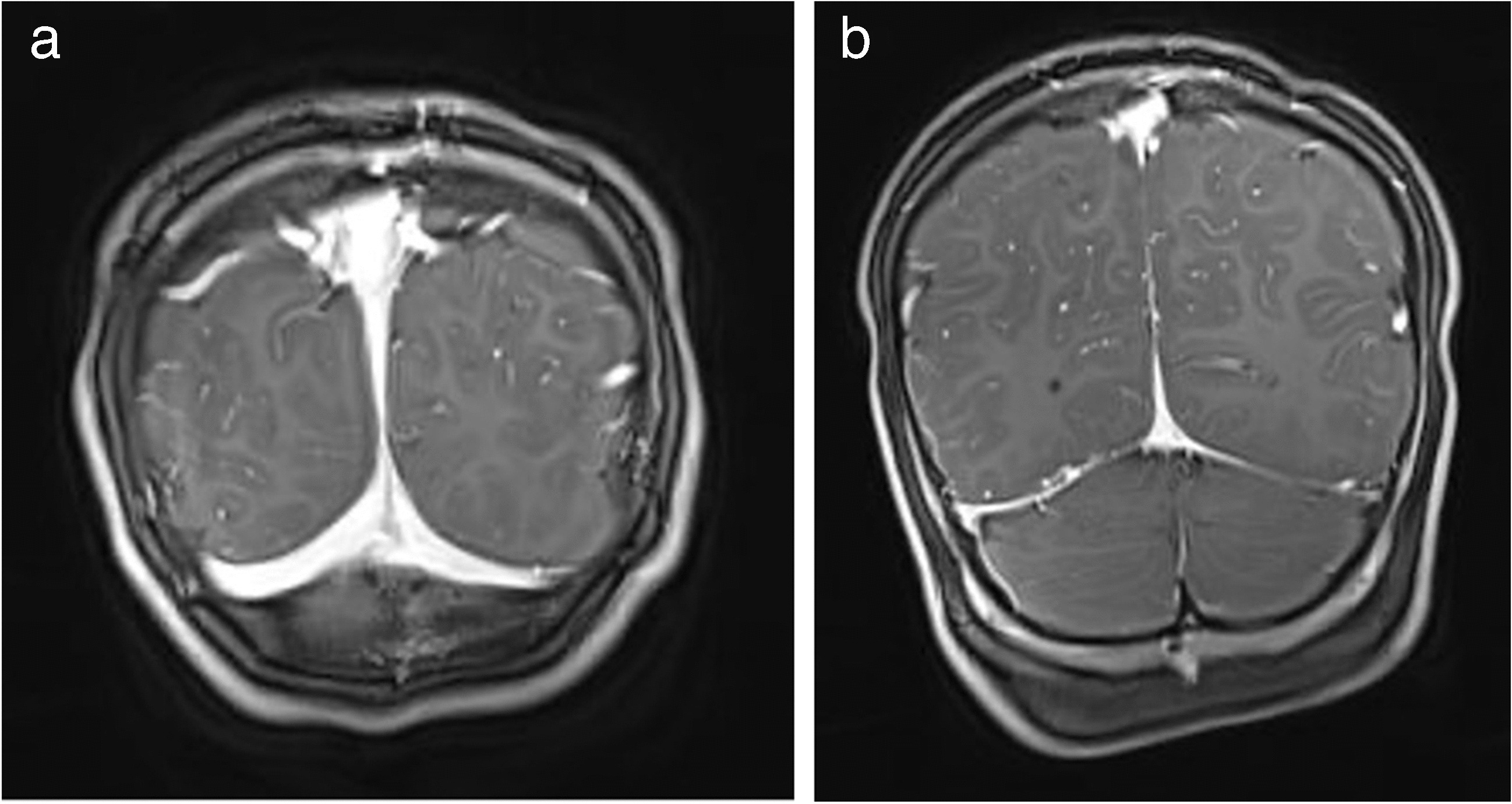
This study consisted of one-hundred-twelve subjects who underwent a clinical routine MRI examination in the context of a full cognitive clinical diagnostic work-up. All consented patients between the ages of 60 and 90 (inclusive) that had a memory consultation at the department of neurology at UZ Brussel between September 2020 and December 2022 were considered for inclusion, irrespective of the severity of cognitive decline. Exclusion criteria consisted of MRI contraindications and structural lesions in the region of interest (temporal lobe). Patient classification was effectuated in compliance with the National Institute on Aging-Alzheimer’s Association criteria for “MCI due to AD” and “Dementia due to AD” [1, 9, 17, 26, 44]. Subjective cognitive decline (SCD) subjects were diagnosed according to the criteria of Jessen’s et al. (2014) [21]. Note that the aforementioned criteria were applied wherever possible, since not all cerebrospinal fluid (CSF) biomarkers were available for the entire study population. Therefore, the final diagnosis used in this study does not necessarily imply a biomarker-based diagnosis. In total, 16 cognitively healthy controls (CN), 33 SCD subjects, 35 mild cognitive impairment patients (MCI), and 27 dementia (DEM) patients were included in this study. Lastly, a randomly selected patient with normal pressure hydrocephalus (NPH) was included to illustrate the effect of a large ILV volume on the MTA score.

MRI acquisition protocol

Brain MRI was performed in all participants using the Philips Ingenia 3T (Philips Medical Systems, Best, The Netherlands). The MRI examination consisted of a sagittal 3D T1-weighted sequence, a sagittal 3D FLAIR-weighted sequence, a coronal T2-weighted sequence, a 3D susceptibility weighted imaging (SWI) and diffusion (DWI). For this study, only the 3D T1-weighted sequence for volumetry and MTA scoring on a coronal reconstruction was used. All scan parameters of the 3D T1-weighted sequence are listed in Supplementary Material Table 1.

Image analysisVisual assessment

The MTA scale by Scheltens, rated on coronal T1-weighted images, was determined individually by three experienced radiologists (G-J. A., T. V., and S. R.), blinded to diagnosis and sex. In case of discrepancy between individual ratings, a consensus MTA score was agreed upon. Images were viewed and evaluated on a Barco (Kortrijk, Belgium) diagnostic screen in AGFA Picture Archiving and Communication System (PACS).

Automated volumetry

From each T1-weighted image, automated brain volumetry was computed by icobrain dm (v 5.10) for total, left, and right hippocampal volumes, as well as for total, left, and right ILV volumes. The initial steps in icobrain dm’s pipeline included skull stripping, bias field correction, and computation of a head size normalization factor as the determinant of an affine transformation to MNI space. The hippocampal and ILV segmentations were obtained with a deep learning-based algorithm trained on a dataset of T1-weighted brain images with high variability both at the population level and in terms of scanners and acquisition parameters [28]. Additionally, a specific intensity-based augmentation strategy that enhances generalizability was used during training [27].

ILV/Hip ratio

An automated alternative of the visual MTA score showed the degree of hippocampal atrophy accounting for volume loss and compensatory expansion of the ILV, defined as the ratio between ILV and hippocampal volumes expressed as a percentage. The ILV/Hip ratio was calculated according to the following formula:

$$\fracratio=\left(\frac^3\right),ILV\right)}^3\right),HC\right)}\right)\times100$$

for each hemisphere (left and right) separately, as well as combined (total).

Normative reference population

In order to integrate the variables age and sex in the interpretation of the ILV/Hip ratio score, a large reference dataset (n = 1903, age range [min–max]: [6–96] years old) comprised subjects without cognitive complaints belonging to 14 different studies with participants derived from open-source data (Supplementary Material Table 2) was used to understand if an individuals’ ILV/Hip ratio score for each patient deviates from the expected score for an individual without cognitive complaints of the same age and sex. Normal aging, derived from the reference dataset, is modeled through univariate interpolating splines, fitted through the percentiles of a shifting age window. Comparing an ILV/Hip ratio score with the trends observed in the subjects without cognitive complaints resulted in a normative percentile adjusted for age and sex. This same methodology was also applied to hippocampal and ILV volumes, creating a percentile score that can be compared to a chosen “cut-off.” Typically, the range between percentile 1 and percentile 99 can be considered a normal range. Any value outside this range might be considered abnormal, which can be used in clinical routine to integrate age and thus evaluate whether a subject’s ILV/Hip ratio score deviates from a healthy aging pattern. A value between the 90 and 99th percentiles can still be considered normal, since this can be inherent to the normal distribution of biological variables, but should nevertheless be interpreted with caution, suggesting that clinical follow-up within 1–2 years might be warranted.

To demonstrate clinical interpretability on patient level, individual cases for each diagnostic category (CN, SCD, MCI, and DEM), as well as the NPH case, were presented. Lastly, an error bar (EB) calculation was performed to evaluate performance specifications, where the error bar interval (− EB and + EB) contains the difference between test and retest values with 90% confidence. This is important since automated measurements can be subject to measurement errors. Therefore, measurement variability should also be considered during result interpretation.

Statistical analysisDescriptive statistics

R environment (R-Studio, v.1.0.136) for statistical computing and graphics was used for all data processing with the following “packages” and (functions). Demographic information was reported as percentages, mean and standard deviation (SD) and/or median and interquartile range (IQR). For categorical variables, the chi-square test of independence was used, while continuous variables were analyzed by the ANOVA test, with a significance level of 0.05 (R package: “arsenal” (tableby and write2word)).

Inter-rater variability analysis

To ensure the quality of the visual assessment for an adequate comparison to automated volumetry, the inter-rater variability was evaluated through the intraclass correlation coefficient (ICC, 95% confidence intervals (CI)), a measure of reproducibility between repeated measurements of the same item, carried out by different observers. (R package “psych” (ICC, v. 2.3.0)). A two-way mixed model, single measurement, with absolute agreement measures was used. The output was the ICC estimate with its respective confidence intervals [38, 43]. The mean ICC and CI were calculated using Fisher’s z transformation (R function: (atanh), to transform the ICC values to z-scores, calculating the mean of the z-scores, and then applying the tanh() function to obtain the mean ICC value.

The ICC is a value going from 0, which indicates no agreement, to 1, indicating absolute agreement, which can be interpreted as either poor (x < 0.50), moderate (0.50 < x < 0.75), good (0.75 < x < 0.90), or excellent (x > 0.90), when taking into account the 95% confidence intervals of the ICC estimate, as suggested by Koo and Li in 2016 [2, 23]. The ICC was calculated using the following formula:

where S2A is the variance among groups, and S2W is the variance within groups [53]. The intra-rater variability was not assessed, as this was beyond the scope of this study.

Association analysis

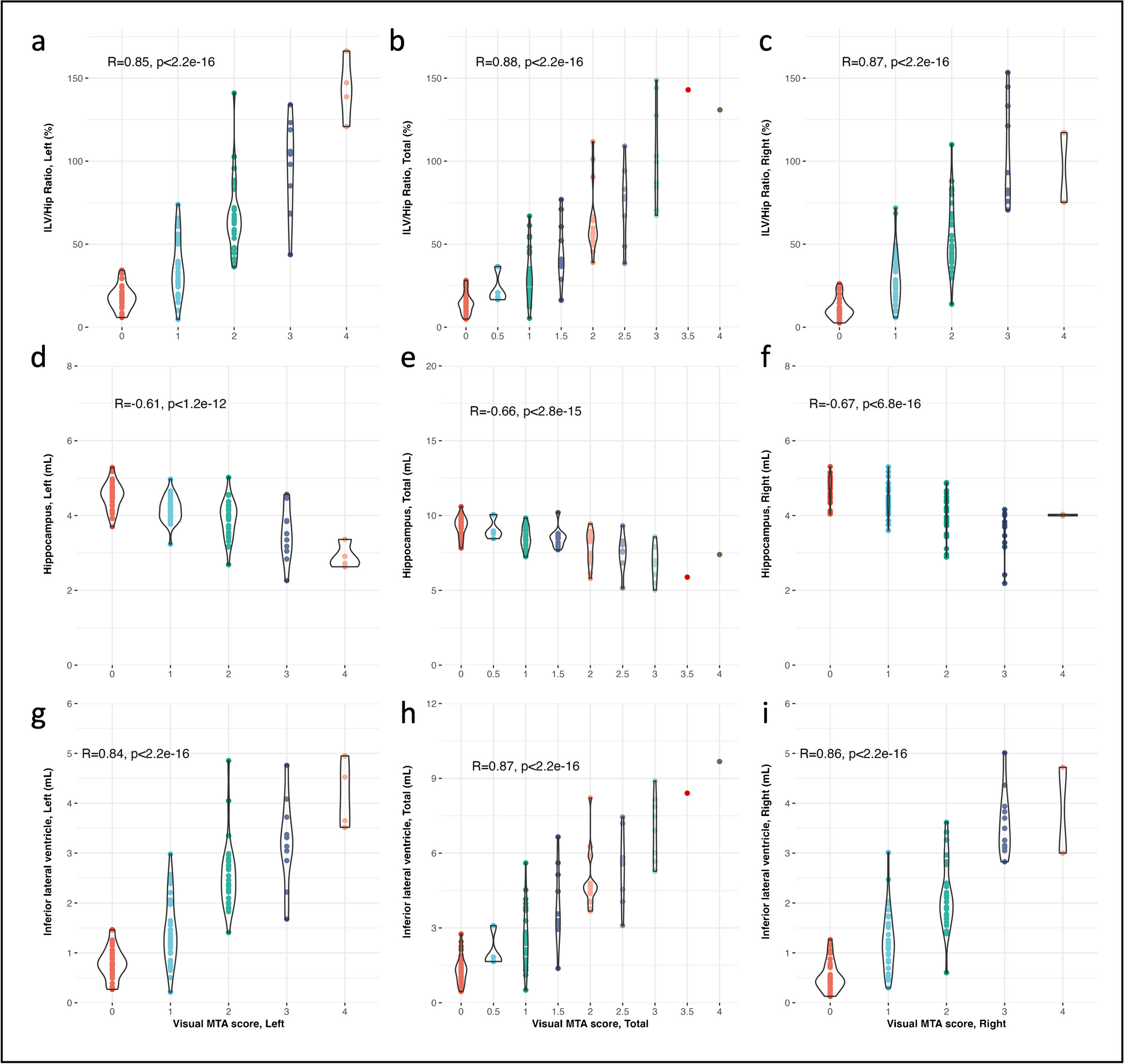
The association between the visual MTA rating (each rater separately and the MTA consensus), cognitive outcome (reflected by the Mini-Mental State Examination, MMSE), and the automated brain segmentations computed by icobrain dm (total, left, and right hippocampal volumes, total, left, and right ILV volumes, and the total, left, and right ILV/Hip ratio) was first quantified using Spearman’s correlation analysis (R package: “base R” (cor)] (alpha < 0.05). Spearman’s rank correlation is a non-parametric measure with robustness to potential non-linearity and outliers, which is often encountered when comparing ordinal (visual MTA) and continuous (automated brain segmentation) variables. Spearman’s values range from − 1 to 1. A value of − 1 indicates a perfect negative monotonic relationship; 0 indicates no monotonic relationship; and 1 indicates a perfect positive monotonic relationship. The strength and direction of the relationship can be interpreted as follows: very weak (|x|< 0.20), weak (0.20 ≤|x|< 0.40), moderate (0.40 ≤|x|< 0.60), strong (0.60 ≤|x|< 0.80), or very strong (|x|≥ 0.80), where a positive value indicates parallel transitions, and a negative value implies an inverse relationship.

Additionally, for a more comprehensive analysis and to not be overly reliant on a single method, Kendall’s Tau (R package: “base R” (cor)] (alpha < 0.05) was used to give more weight to the ordinal nature of the visual MTA ratings and to examine the concordance between the automated measurements and visual MTA ratings. Kendall’s Tau, like Spearman’s correlation, is a versatile measure that ranges from − 1 to 1, where − 1 indicates a perfect negative association; 0 implies no association; and 1 signifies a perfect positive association. The strength and direction of the association can be summarized as very weak (|x|< 0.10), weak (0.10 ≤|x|< 0.30), moderate (0.30 ≤|x|< 0.50), strong (0.50 ≤|I|< 0.70), or very strong (|x|≥ 0.70).

Moreover, a logistic regression was performed (R package: “rms” (lrm)) to further evaluate the relationship between the visual MTA as outcome and the automated brain segmentations as predictor. Various additional scale invariant metrics, including the concordance index (c-index/area under the curve (AUC)) and the Brier score, were used to further quantitatively evaluate the strength, direction, degree of association, and correlation.

The AUC assesses how well the model distinguishes between the different visual MTA severity scores based on the predicted probabilities. The AUC varies being 0 and 1, whereas a general guideline AUC > 0.90 signifies excellent discrimination, 0.80 ≤ AUC < 0.90 represents good, 0.70 ≤ AUC < 0.80 denotes moderate to good, 0.60 ≤ AUC < 0.70 reflects moderate to poor, and AUC < 0.60 indicates very poor discrimination. AUC equals 0.50 indicates no discriminative power (random chance). Thus, a high AUC suggests the model is effective at ordering and ranking cases according to MTA severity and would indicate that both scoring methods provide very similar rankings, and by extension, high correlation, encouraging the prospects for interchangeability.

The Brier score quantifies the accuracy of predicted probabilities, where a low Brier score suggests accurate predictions, further reinforcing correlation between the two variables. A Brier score ≤ 0.2 indicates excellent model performance; 0.2 < Brier score ≤ 0.25 reflects a good; 0.25 < Brier score ≤ 0.3 suggests a fair; 0.3 < Brier score ≤ 0.35 signifies poor; and a Brier score > 0.35 implies very poor model performance.

Even though these additional metrics do not offer a traditional correlation coefficient, they do offer information about the quality of predictions and alignment between predicted and actual values, which indirectly reflects the degree of correlation.

Classification accuracy

To determine whether the ILV/Hip ratio exhibits comparable diagnostic precision or provides additional information compared to other measurements, classification accuracy through logistic regression of the visual MTA ratings (each rater separately and the MTA consensus) and the automated volumetric measurements (total, left, and right hippocampal volumes, total, left, and right ILV volumes, and the total, left, and right ILV/Hip ratio), was conducted for each variable separately as predictors. The following pairwise combinations of disease stages were considered as binary outcomes: SCD vs. CN, MCI vs. CN, DEM vs. CN, MCI vs. SCD, DEM vs. SCD, and DEM vs. MCI.

Classification performance was evaluated using receiver operating characteristic (ROC) analysis, with the R package “pROC” (roc, auc, coords, and ci) and the “stats” (predict and glm) package [40]. AUC, sensitivity, specificity, positive predictive value (PPV), and negative predictive value (NPV), were documented for each pairwise combination of disease stages. The AUC was computed with the trapezoidal rule. The Youden index to determine the threshold that maximizes the distance to the identity (diagonal) line, from which the sensitivity, specificity, PPV, and NPV were calculated. In addition, for each binary classification, resampling with replacement to estimate the variability of the AUC was employed. The resulting bootstrapped-based confidence intervals were then used to investigate if the AUC values between the variables were significantly different.