1 Introduction

Inspired by brain science, Spiking Neural Networks (SNNs) use binary spikes to transmit information, which are event-driven, and offer low energy consumption and high biological plausibility. SNNs are regarded as the next generation of neural networks (Maass, 1997). However, current SNNs are still suffering from insufficient performance. Complex patterns of neuronal connections within and across brain regions, along with specialized neuronal architectures for particular functions, enable the brain to adeptly handle information processing across diverse scenarios (Luo, 2021). Information processing in visual pathways can be modeled by convolutional structure (Fukushima, 1980). In visual pathways, a neuron receives spikes from presynaptic neurons within its receptive field and processes the incoming information in the soma. However, the difference is that the process of convolution operation in Convolutional Neural Networks (CNNs) is analogous. The receptive field in CNNs is determined by the size of the convolution kernel. Recent researches indicate that certain neuronal connections share functional similarities with the transformer architecture (Vaswani et al., 2017). Specifically, a network composed of astrocytes, neurons, and tripartite synapses between them, was proven to naturally implement the core operations of transformer structure (Kozachkov et al., 2023). Moreover, a recent study revealed that the transformer functions are similar to the hippocampus, when equipped with recursive positional encoding, the transformer structure can accurately replicate the spatial representation of hippocampal formation (Whittington et al., 2021). Integrating convolutional and transformer structures in SNNs can help process both local and global information simultaneously, potentially improving the performance of SNNs. In the realm of artificial neural networks (ANNs), a similar idea was adopted in various models (Chen et al., 2022; Guo et al., 2022; Peng et al., 2023).

Convolution-based SNNs are suitable for vision tasks, with their inherent translational invariance and inductive bias. However, the training of SNNs is challenging due to the non-differentiable nature of their activation functions. Surrogate Gradient (SG) method (Neftci et al., 2019), replacing the original non-differentiable step function in neurons with a differentiable function during backpropagation, simplified the training of convolution-based SNNs. Gradient vanishing and explosion significantly impede the scaling and performance enhancement of SNNs. The application of residual connections and some normalization techniques (He et al., 2015; Fang et al., 2021a; Zheng et al., 2021; Hu et al., 2023a) demonstrated substantial effectiveness in enhancing network depth and performance. Specifically, threshold-dependent batch normalization (tdBN; Zheng et al., 2021) was proposed to alleviate the problems of gradient vanishing and explosion, and successfully applied to train convolution-based SNNs up to 50 layers. Furthermore, Spike-Element-wise (SEW) ResNet (Fang et al., 2021a) further mitigated the gradient vanishing and explosion problem, obtaining a directly trained SNN beyond 100 layers for the first time, and achieved notable top-1 accuracy on the ImageNet dataset. Despite these breakthroughs, Convolution-based SNNs still suffer to meet the evolving demands of complex computational tasks.

Vision Transformer (ViT; Dosovitskiy et al., 2020) showed superior performance in a wide range of vision tasks. This success led to increased interest in integrating transformer architectures with SNNs. Spikeformer (Li et al., 2022) utilized spatial-temporal self-attention to extract global features in both spatial and temporal domains. However, Spikeformer struggled with a high computational load due to numerous floating-point multiplications and exponential operations in softmax. Spikformer (Zhou Z. et al., 2023) proposed spiking self-attention (SSA), innovatively eliminating the softmax function, and reducing computational complexity while enhancing performance. Moreover, based on the Spikformer, other spiking transformers were developed to improve the performance, such as Spikingformer (Zhou C. et al., 2023) and Spike-driven Transformer (Yao et al., 2023a). However, there remains a performance gap when comparing spiking transformers to their ANN counterparts, suggesting an ongoing opportunity for further development.

In this study, to address the challenge of limited performance, we propose a directly trained SNN that integrates convolutional structure and transformer structure, named Spiking Global-Local-Fusion Transformer (SGLFormer). In addition, we uncover the issue of inaccurate gradient backpropagation induced by inappropriate Maxpooling operations in SNNs, which hampers the performance. This is addressed by the development of an SNN-optimized Maxpooling module. Moreover, the spatio-temporal block (STB) is employed in the classification head to aggregate spatial and temporal features effectively. Experimental results show that various components of SGLFormer collaboratively contribute to improving its performance. SGLFormer achieves high performance on both static and dynamic vision sensor (DVS) datasets, especially on ImageNet, with a top-1 accuracy of 83.73%, significantly surpassing existing SOTA methods.

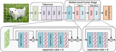
2 Method 2.1 The overall framework of SGLFormer

Inspired by the biological neural system, we integrate the convolutional structure and the transformer structure in SNNs to construct the high-performance SGLFormer. The overall framework of SGLFormer is shown in Figure 1. The SGLFormer includes a Tokenizer module, a Global-Local-Fusion Stage, and a linear classification head. The neuron used in SGLFormer is LIF (Leaky Integrate-and-Fire), which is simple but retains biological characteristics. The dynamics of LIF are described as Equations (1–3):

H[t]=V[t-1]+1τ(X[t]-(V[t-1]-Vreset))    (1) S[t]=Θ(H[t]-Vth)    (2) V[t]=H[t](1-S[t])+VresetS[t]    (3)

where τ in Equation (1) is the membrane time constant, X[t] is the input current at time step t. Vreset represents the reset potential, Vth represents the spike firing threshold, H[t] and V[t] represent the membrane potential before and after firing spike at time step t, respectively. Θ(v) is the Heaviside step function, if v ≥ 0 then Θ(v) = 1, means that firing a spike, otherwise Θ(v) = 0. S[t] represents the output of neuron at time step t.

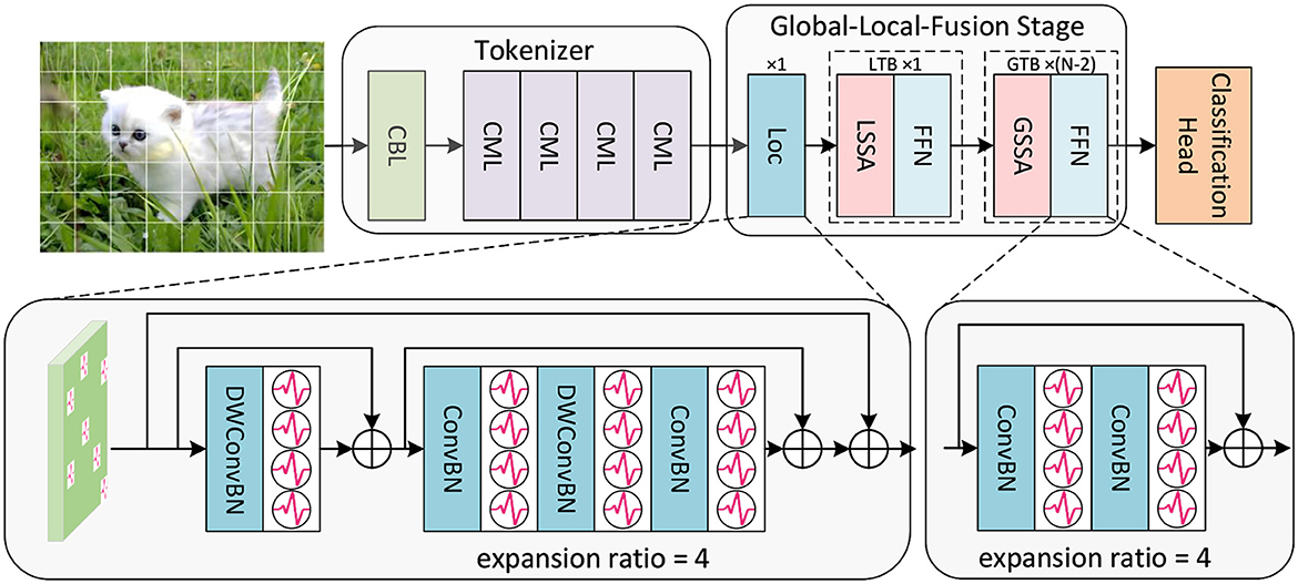
Figure 1. The overall framework of SGLFormer, which consists of a Tokenizer module, a Global-Local-Fusion Stage, and a linear classification head. LTB is a local transformer block, and GTB is a global transformer block.

Given a 2D image sequence I∈ℝT×B×3×Hinput×Winput (or a neuromorphic event sequence I∈ℝT×B×2×Hinput×Winput), T is time steps, and B is batch size. The Tokenizer module contains 1 CBL and 4 CMLs. CBL is the abbreviation of ConvBN-LIF, and CML is our SNN-optimized Maxpooling to address the problem of inaccurate gradient backpropagation caused by inappropriate Maxpooling in SNNs. The Tokenizer module is used for feature extraction, channel dimension expansion, and patch embedding. The output of the Tokenizer is XToken∈ℝT×B×C×H×W.

Each Global-Local-Fusion Stage contains N blocks. The number of local feature extraction block Loc and local transformer block (LTB) are both 1, and the number of global transformer block (GTB) is N − 2. The LTB consists of local spiking self-attention (LSSA) and feedforward network (FFN), and the GTB consists of global spiking self-attention (GSSA) and FFN. The classification head employs STB instead of global average pooling, which facilitates the aggregation of spatial and temporal features. The overall framework of SGLFormer with N = 3 is expressed as Equations (4–8):

XToken=Tokenizer(I),   I∈ℝT×B×3×Hinput×Winput    (4) XLoc=Loc(XToken),   XToken∈ℝT×B×C×H×W    (5) XLTB=FFN(LSSA(XLoc)),   XLoc∈ℝT×B×C×H×W    (6) XGTB=FFN(GSSA(XLTB)),   XLTB∈ℝT×B×C×H×W    (7) Y=Classify(XGTB),   XGTB∈ℝT×B×C×H×W,Y∈ℝC    (8)

In the above equations, Hinput, Winput, H, and W are the height of the input data, the width of the input data, the height of the intermediate feature maps, and the width of the intermediate feature maps, respectively, and C is the number of channels and the embedding dimension of the SGLFormer. Classify(·) denotes the classification head operation.

2.2 Global-Local-Fusion Stage

The primary visual cortex in the brain mainly extract local information, while the higher-level brain regions focus on abstract high-level information. Based on this, we propose a Global-Local-Fusion Stage that integrates local feature extraction first and then global self-attention. Loc, LTB, and GTB together constitute the Global-Local-Fusion Stage. Loc contains convolution and depthwise convolution, and the expansion ratio controls the number of feature map channels. For example, if the expansion ratio is 4, the convolution layer in Loc will first lift the number of channels to C × 4, and then drop back to the original number of channels C. The FFN in LTB and GTB, like that in the Loc, controls the number of channels by the expansion ratio. GSSA in GTB is equal to SSA in Spikformer, which is global spiking self-attention. With the input feature map XinputG∈ℝT×B×C×H×W, the computation of GSSA (SSA) is as Equations (9–12):

Q′=CBLQ(XinputG),   K′=CBLK(XinputG),   V′=CBLV(XinputG)    (9) Q,K,V=Reshape(Q′,K′,V′),   Q′,K′,V′∈ℝT×B×C×H×W    (10) XGSSA′=Reshape(LIF(QKTV×f)),   Q,K,V∈ℝT×B×C×N    (11) XGSSA=CBL(XGSSA′),   XGSSA,XGSSA′∈ℝT×B×C×H×W    (12)

where CBL(·) is ConvBN-LIF, in which the convolution kernel size is 1 × 1 and stride is 1, and f is scaling factor, N = H × W is the number of tokens.

LSSA in LTB is local spiking self-attention, of which the schematic diagram is shown in Figure 2. In the LSSA block, the input feature map XinputL∈ℝT×B×C×H×W is first partitioned into 2 × 2 small feature maps, and the height and width of each small feature map are H2 and W2, respectively. After that, spiking self-attention is calculated in each partitioned small feature map. The parameters of spiking self-attention for each partitioned small feature map are shared to reduce computational cost. The small feature maps are then restored to original size for integration. The computation of LSSA is as Equations (13–15):

XPartition,i=Partition(XinputL),   i∈[1,4]    (13) XSSA,i=SSA(XPartition,i),   XPartition,i,XSSA,i∈ℝT×B×C×H2×W2    (14) XIntegration=Integration(XSSA,1,XSSA,2,XSSA,3,XSSA,4)    (15)

where XIntegration∈ℝT×B×C×H×W is the output feature map of LSSA.

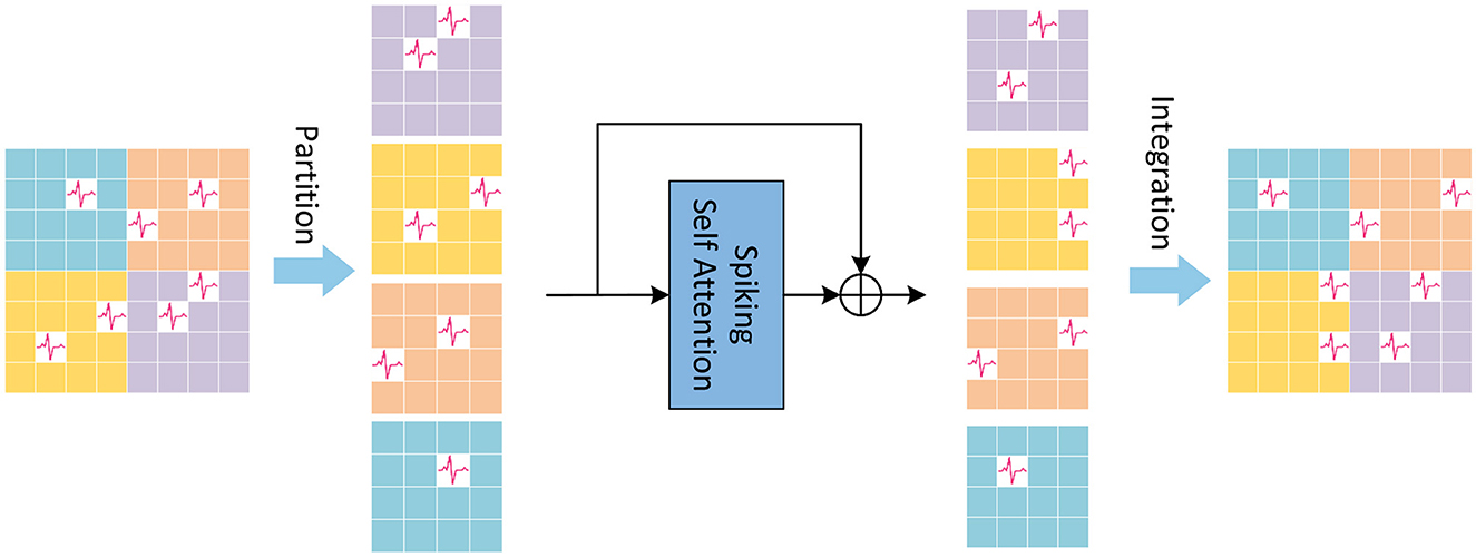
Figure 2. The Local Spiking Self Attention (LSSA), which first divides the feature map into four equally sized parts, and integrates it into the original size after spiking self-attention calculation performed inside the divided feature map.

2.3 SNN-optimized Maxpooling: CML

We observe that the existing downsampling in SNNs yields inaccurate backpropagation gradients, which can hamper the development and performance improvement of SNNs. We address the problem of inaccurate gradient backpropagation in SNNs by CML.

2.3.1 Inaccurate gradient backpropagation

SNNs typically employ the network module shown in Figure 3A, i.e., ConvBN-LIF-Maxpooling (CLM), which gives rise to the problem of inaccurate gradient backpropagation. ConvBN represents the combination of convolution and batch normalization. Following ConvBN are the spiking neurons, which receive the resultant current, accumulate the membrane potential across time, and fire a spike when the membrane potential exceeds the threshold. Maxpooling is performed after spiking neurons for downsampling. The output of ConvBN, spiking neurons, and Maxpooling layers, are feature maps x ∈ ℝm × n, h ∈ ℝm × n, and y∈ℝms×ns respectively, where s is the pooling stride.

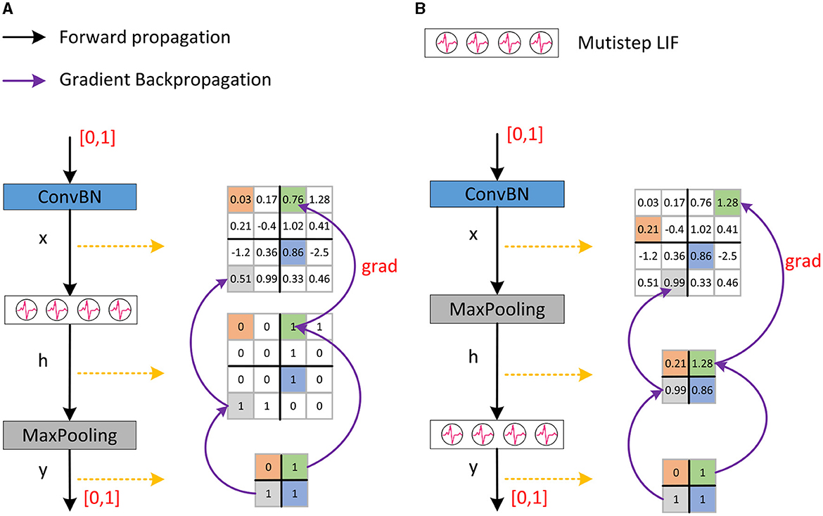
Figure 3. The downsampling method in Spikformer and our proposed SNN-optimized Maxpooling. (A) Shows the downsampling method in Spikformer which has an inaccurate gradient backpropagation issue. (B) Shows our proposed SNN-optimized Maxpooling (CML) with accurate gradient backpropagation.

Given the loss function L and the backpropagation gradient ∂L∂yij after downsampling, the gradient at the feature map x is as Equation (16):

∂L∂xuv=∑i=0ms∑j=0ns∂L∂yij∂yij∂huv∂huv∂xuv    (16)

The backpropagation gradient of Maxpooling is as Equation (17):

∂yij∂huv={1,huv=max(hi×s+k,j×s+r)0,others    (17)

where k, r ∈ [0, s). The backpropagation gradient of the LIF neuron is:

∂huv∂xuv=∂S[t]∂X[t]=