1 Introduction

Electroencephalogram (EEG) is a method for detecting brain signals (Ismail et al., 2016). It uses tiny electrodes attached to the scalp to detect electrical activity in the brain. The EEG signals generated by brain thinking activity can be analyzed and processed by corresponding analysis algorithms, and then converted into corresponding commands to control computers or electronic devices (Hramov et al., 2021).

In recent years, non-invasive brain–computer interfaces (BCI) have achieved significant results in the acquisition of EEG signals (Galán et al., 2008). BCI have been applied in many fields such as sleep signal acquisition, disease diagnosis, emotion analysis, and robot control, which have broad application prospects (Allison et al., 2007).

The application of EEG in monitoring sleep quality is also essential (Sadeh, 2015). Sleep staging can monitor the quality of each sleep segment and determine a person's sleep quality (Carskadon et al., 2005). In the auxiliary diagnosis of some sleep-related diseases such as epilepsy and sleep apnea, sleep staging plays an important role in the diagnosis of the disease (Samy et al., 2013) and can help improve our analysis of these related diseases. The identification of sleep stages is crucial for the diagnosis of sleep disorders, among which obstructive sleep apnea (OSA) is one of the most common diseases (Korkalainen et al., 2019). Traditional manual sleep staging using EEG signals is time-consuming and laborious since it requires analyzing sleep stages from the entire night's sleep signal.

In recent years, a research method for EEG sleep staging using deep learning algorithms has been proposed. Deep learning is a new research direction in the field of machine learning (Arel et al., 2010). It is introduced into machine learning to make it closer to its original goal of artificial intelligence (AI) (Arrieta et al., 2020). Deep learning is a complex machine learning algorithm that learns the internal rules and representation levels of sample data. The information obtained during the learning process is very helpful for interpreting data such as text, images, and sound (LeCun et al., 2015; Tsinalis et al., 2016). The ultimate goal is to enable machines to analyze and learn like humans and recognize data such as text, images, and sound. Deep learning is a powerful tool in the processing of EEG signals and has shown excellent performance in speech and image recognition (Amin et al., 2019; Sun et al., 2019). Traditional EEG sleep staging algorithms include deep learning algorithms or end-to-end trained deep learning algorithms, including convolutional neural network (CNN) or recurrent neural network (RNN) algorithms (Dong et al., 2017; Chambon et al., 2018; Phan et al., 2018; Perslev et al., 2019; Qu et al., 2020), involving state-of-the-art sleep staging networks such as DeepSleepNet (Supratak et al., 2017) and SeqSleepNet (Phan et al., 2019).

The traditional approach to deep learning research involves obtaining a large dataset for a specific task and training a model from scratch using that dataset (Dietterich, 1997). Although deep learning models can achieve high accuracy, the training time and computational cost of this method are significant due to the requirement for large amounts of data (Alzubaidi et al., 2021). In the case of unfamiliar subjects, using deep learning algorithms would require re-calculating, which would consume a considerable amount of computational time and resources. Furthermore, data from different cohorts may come from varying sources due to variations in the number and location of EEG channels, sampling frequency, experimental paradigms, and subject variability, making models trained on one cohort not directly applicable to another, limiting their applicability in clinical settings (Boostani et al., 2017; Andreotti et al., 2018).

Meta-learning, also referred to as learning to learn, involves a systematic examination of the performance of various machine learning methodologies across a diverse spectrum of learning tasks. This process enables the acquisition of knowledge from the amassed meta-data, allowing for significantly accelerated learning of novel tasks beyond conventional capabilities (Vanschoren, 2019). This not only expedites and enhances the development of machine learning workflows and neural network architectures but also facilitates the replacement of manually engineered algorithms with innovative data-driven approaches. Yaohui Zhu proposed a multi-attention meta-learning (MattML) method for few-shot finegrained image recognition (FSFGIR) (Zhu et al., 2020). Instead of using only base learner for general feature learning, the proposed meta-learning method uses attention mechanisms of the base learner and task learner to capture discriminative parts of images.

Meta-learning algorithms can enable cross-subject EEG sleep staging, greatly reducing the training time required for sleep staging. Nannapas proposed a meta-learning MAML-based method, MetaSleepLearner, for sleep staging EEG signals (Finn et al., 2017; Banluesombatkul et al., 2020). They introduced a transfer learning framework based on model-agnostic meta-learning (MAML) to transfer acquired sleep stage knowledge from a large dataset to new individual subjects. The accuracy achieved on the Fpz-Cz validation channel was 72.1% and the MF1 score was 64.8, demonstrating the feasibility of cross-subject EEG sleep staging. Shi et al. (2023) used meta-transfer learning, proposed MTSL, further improved the feature extracter based on the meta-learning framework, and introduced the idea of transfer learning to improve the performance of sleep staging in small sample scenarios through a new meta-transfer framework, and achieved 79.8% ACC on sleep-EDF. In MetaSleepLearner, the experiment uses too many training sets for hybrid training and requires fine-tuning on unused subject data, so the complexity of the experiment does not favor a specific implementation. In MTSL, a multi-stream parallel CNN network is used to extract EEG features from each of the three scales, and finally, the multi-scale features are fused through feature splitting to obtain the final EEG feature representation. Since the network features are too complex, the running time and computational consumption are too large and difficult to implement.

In this study, we propose a few-shot EEG sleep staging based on transductive prototype optimization network (TPON) method to improve the accuracy of cross-subject EEG sleep staging. The aim is to improve the performance of cross-subject EEG sleep staging and also to achieve innovative cross-channel recognition of sleep with good performance. Our experiments are carried out with 20 subjects in the Sleep-EDF dataset, which has a small amount of data and moderate network complexity. We use the prototype network model in meta-learning. Compared with traditional machine learning and other meta-learning methods, our experiment has shorter training time and higher accuracy improvement. Our experiment is based on the prototype network method of meta-learning proposed by Snell et al. (2017). To improve it, we utilize the Transductive Distribution Optimization (TDO) algorithm proposed by Liu et al. (2023). Our experiment is conducted on the Fpz-Cz and Pz-Oz channels and uses the AASM (Berry et al., 2012) scoring standard, which classifies sleep into five stages.

The main contributions of this study are as follows:

• We propose a few-shot EEG sleep staging based on transductive prototype optimization network (TPON) method to improve the performance of cross-subject EEG sleep staging.

• By using few-shot learning and TPON method, we effectively alleviated the problem of too few samples in sleep staging and improved the generalization ability to new subjects.

• In the five-way 15-shot scenario, the cross-subject sleep staging accuracy of TPON can be improved to 87.1%, MF1 to 81.7, and the cross-channel sleep staging can also achieve an accuracy of 82.4%. Additionally, we first experiment and discuss the feasibility of cross-channel sleep staging recognition.

2 Proposed method

In this study, we propose a few-shot EEG sleep staging based on transductive prototype optimization network (TPON) method to improve the accuracy of cross-subject EEG sleep staging. Our experiments are based on the prototypical network approach of meta-learning, where prototypes are used in combination with high confidence unlabeled samples to achieve subject transfer.

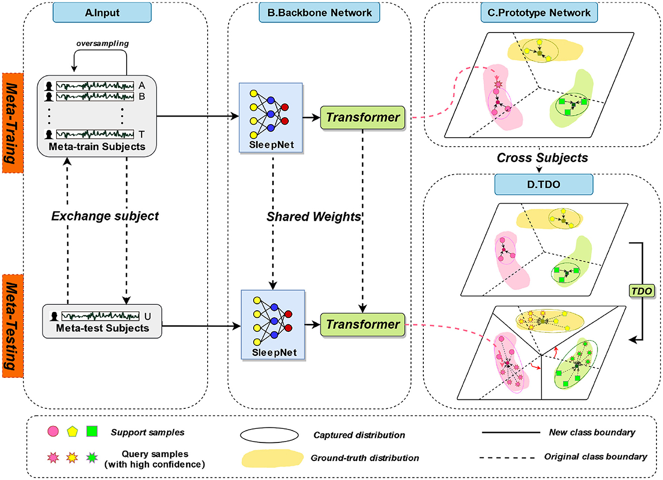
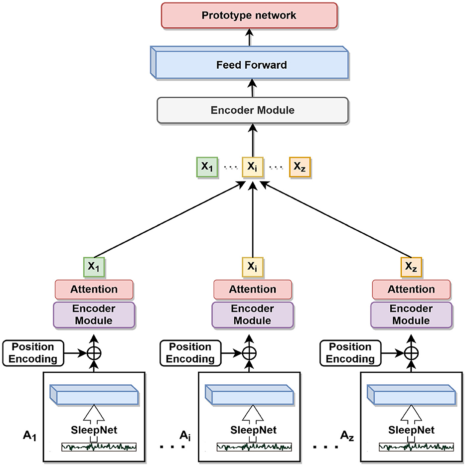
2.1 Overall framework of TPON

The overall framework of TPON is depicted in Figure 1. Different subjects will be used for both meta-training and meta-testing, which is shown at stage A in Figure 1, 19 of them for meta-training and the remaining one for meta-testing. In the meta-training phase, we combine the sleep data of 19 meta-training subjects. Each participant had two nights of data. In the meta-testing phase, data from two nights of one meta-testing subject are combined. We also cross-tested 20 times to obtain average results for all subjects. During meta-testing and meta-training, the sleep network shares the weight values. In the meta-training stage, prototypes of five sleep cycles are obtained through 50 experiments and randomly averaged sampling. Then, during our meta-testing phase, unlike meta training, due to the few-shot size of the meta-testing set.

Figure 1. The overall framework of TPON.

Phase B in Figure 1 is the backbone network we used, including SleepNet combined with Transformer. The C and D stages in Figure 1 are the improved prototype network and transformation distribution optimization (TDO) methods we used, respectively. The mentioned three phases are discussed in detail in the following sections.

We utilizing the various distance metric functions, including the Cosine distance formula, the Manhattan distance formula, the Euclidean distance formula, and the Chebyshev distance formula. By comparison, we then obtain the highest accuracy among the four. We identify the class to which a test EEG data segment belongs based on its proximity to the prototype. We then compute the average accuracy, precision, loss, and F score for each of the five categories.

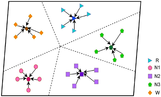
2.2 Prototypical networks

In this study, we focus on the prototypical network approach, which is shown in Figure 2 and stage C in Figure 1. The method is based on the classification of sleep EEG signals. We have developed our prototypical network model, which maps sleep EEG signals to embedding vectors and uses their clustering for classification (Hori et al., 2001). The novel feature of our model is that it constructs a richer embedding space through a learned prototypical network related to EEG sleep, such that EEG signals can be projected there. In the Figure 2, we show the five-way five-shot during the five periods of sleep. They are clustered under a distance metric of orientation and class relevance, which is then used for classification (Schultz and Joachims, 2003; Chen et al., 2009).

Figure 2. Prototypical network.

In few-shot learning (Sung et al., 2018; Wang et al., 2020), if our task is an N-way K-shot, then the support set S, with K-labeled samples, can be expressed as follows:

S={(X1,Y1),(X2,Y2),…,(XN,YN)}    (1)

Each prototype is an average vector of embedded support points belonging to its class. To better represent the features of each class, the average value of the features of each class is computed by the backbone network F, which is called the prototype Cq. Under the K-shot dimension, xi∈ is the eigenvector of class i, and i is any one of the N classes, yi∈ are the labels of the corresponding category. Then, Sq respectively represent the support set of class q. |Sq| is expressed as the absolute value of Sq. The calculation formula is as follows:

Cq=1|Sq|∑(xi,yi)∈SqF(xi),    (2)

Based on the distance from the embedding space to the prototype, the distance metric function d is given, the prototypical network generates a distribution over classes for the query point x using a softmax activation function, which is computed as follows :

P(y=q|x)=exp(−d(F(xi),Cq))∑q′exp(−d(F(xi),Cq′)),    (3)

Specifically, P(y = q|x) means that the query sample x is compared to all Cq′ prototypes, classifying x as a probability value of class q.

A common prototypical network consists of an backbone network that maps sleep EEG signals to embedding vectors. One batch contains a subset of the available training EEG signals. EEG data from each class is randomly split into support and query sets. The embedding of the support set is used to define the class prototype, i.e., the prototype embedding vector of the class. By using a metric function to measure the distance between the query set and the prototype, the query set is classified.

2.3 Distance metric

For prototypical networks and matching network, any measurement function is allowed. In our experiment, dCos means Cosine distance, dMan means Manhattan distance, dEuc means Euclidean distance, and dChe means Chebyshev distance, they were used as comparisons. We obtain the cosine distance as our best matching and most accurate measurement function.

If there is a query sample Zf, its high-dimensional spatial characteristics can be expressed F(Zf), and n represents the dimension of the vector. Therefore, the distance function can be used to obtain the distance between the high-dimensional vector F(Zf) of our query sample and the prototype Cq. The distance calculation formula is as follows:

dCos(F(Zf),Cq)=-cosθ=-F(Zf)·Cq||F(Zf)||||Cq||,    (4) dMan(F(Zf),Cq)=∫k=1n|F(Zf,k)−Cq,k|,    (5) dEuc(F(Zf),Cq)=(∫k=1n|F(Zf,k)−Cq,k|2)12,    (6) dChe(F(Zf),Cq)=MAXf|F(Zf)−Cq|,    (7)

After the Cosine distance between the query sample and the prototype Cq is obtained, the negative value of the Cosine distance between the query sample Zf and the prototype Cqis formed into a probability distribution on the class through the softmax function. The calculation formula is as follows:

P(yn∣Zf)=exp(−dist(F(Zf),Cq))∑n=1qexp(−dist(F(Zf),Cq′)),    (8)

where Cn(n = 1, 2, …, Q) is the prototype of class n and dist() can represent four different distance measurement functions.

At the same time, to have a good evaluation index during model training, the experiment uses cross entropy as loss function to train and then minimizes the loss function. The calculation formula is as follows:

Loss=-1n∑i=1n∑n=1qyin×log(p(yn∣Zf)),    (9)

where n is the number of query samples and yi is the actual label of the sample.

2.4 Transductive distribution optimization

Due to the small number of subjects per sleep period in the sleep data SleepEDF-2013, the problem is that the selected sleep segments do not accurately describe our actual prototypes. To solve this problem, we used the TDO method based on the original prototype network.

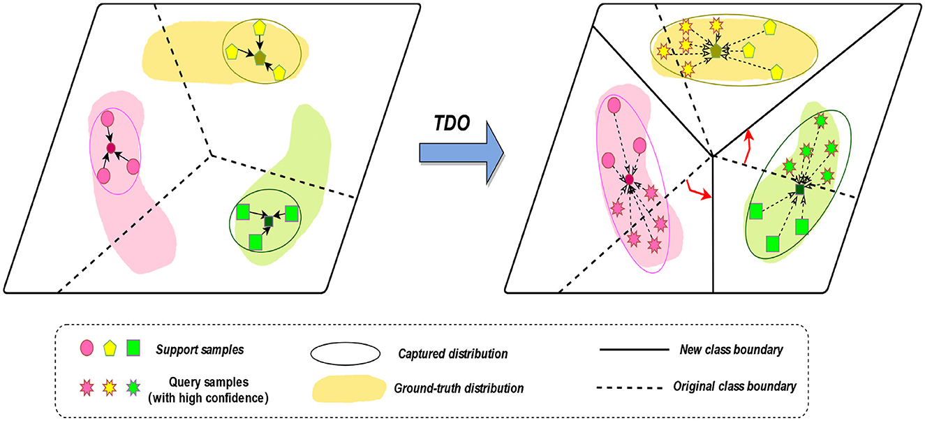
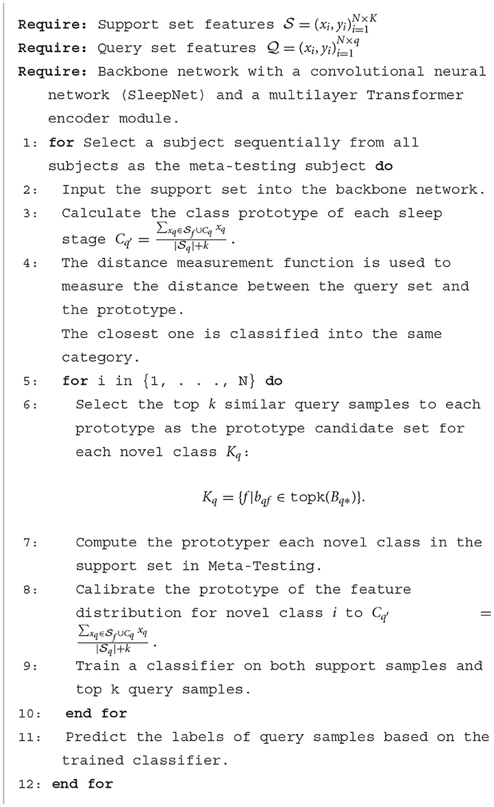
We propose to use the prototype network approach of TDO to capture the features of new classes. We first used the original method, using labeled samples from the five sleep epochs as a support set, to obtain prototypes of the five sleep epochs. However, due to the small number of samples in the learning process, it is not possible to accurately obtain the true distribution of each class. Therefore, we introduce TDO, which combines support set and high-confidence unlabeled sample query set to improve the matching degree of prototypes in prototype network, which is depicted in Figure 3 and stage D in Figure 1. Algorithm 1 summarizes the prediction process of our proposed method.

Figure 3. The transductive distribution optimization (TDO) method.

Algorithm 1. Transductive prototype optimization network (TPON) algorithm.

The main steps are illustrated in the figure above, which include the following three parts:

2.4.1 Generate an original class boundary

In the first stage, we generate an original class boundary using the backbone network and the labeled data. The feature extraction prototype network extracts an original prototype for a five-way N-shot task by using the backbone network, generating an original class boundary, where all the support set samples come from labeled data. For an N-way K-shot task, to find out the similarity scores between all query samples and the support classes, we use the sample-to-class metric measure to get the relational matrix R(N × q) × N of similarity probability scores.

2.4.2 Generate a new class boundary

The class distribution is optimized by using a robust feature extractor to capture the feature distribution of each class. It is based on the original support set and some highly confident unlabeled query samples to obtain a ground-truth prototype of the transformed distribution. New class boundaries are generated by combining the original support set and some highly confident unlabeled query samples. The goal is to generate a new classifier that predicts the labels of all remaining query samples.

Then, we obtain a similarity probability score matrix B∈R(N × q) × N between each prototype Cq and all query samples Zf. For each class prototype Cq, we select the top k query samples with the highest similarity probability score as the prototype class candidate set:

Kq={f|bqf∈topk(Bq*)},Cq={xq|xq∈Q,q∈Kq},    (10)

topk(·) is an operator to select the top k elements from each row of the matrix B, k is a hyperparameter that denotes the number of samples in the prototype class candidate set for each class, and Q denotes the query set after Tukey's transformation. Ki stores the index of the k most similar query samples of class i and Ci stores the samples corresponding to Ki.

2.4.3 Generate a new classifier

A new classifier is generated by combining the original support set and some highly confident unlabeled query samples to generate new class boundaries. With the goal of predicting the labels of all remaining query samples, the mean of the feature distribution for each class is then computed using the support set and the candidate set of prototype classes:

Cq′=∑xq∈Sf∪Cqxq|Sq|+k,    (11)

where |Sq| denotes the number of samples in Sq and k denotes the number of samples in Cq. This significantly removes the distribution bias caused by the category mismatch. Our method does not introduce any additional rational parameters and can be paired with most classification models and feature extractors. The introduction of this approach does not add a significant amount of computation, but it can greatly improve the classification accuracy and achieve significant learning results.

3 Dataset and experimental setup

In this section, we present the details of our experiments on the proposed method, including dataset and experimental setup. For our experiments, the hardware and software configurations used in our experiments are based on a platform with an Nvidia RTX 3090Ti, Ubuntu 16.04, and PyTorch 1.9.0.

3.1 Datasets

This section describes the use and preprocessing of the experimental data. The experiment used the benchmark sleep data disclosed by PhysioNet Sleep-EDF, which included 20 healthy subjects (26–35 years old), including 10 healthy men and 10 healthy women. The polysomnography (PSG) recording time of each person is about 20 h. This dataset includes sleep EEG of healthy subjects' SC. The * PSG.edf as the suffix contains EEG (from Fpz-Cz, Pz-Oz electrode positions) and the * Hypnogram.edf files contain the notes of sleep mode corresponding to PSG. The sampling rate was 100 Hz for all EEG.

Sleep experts manually divide these records into eight categories (W, N1, N2, N3, N4, REM, MOVEMENT, and UNKNOWN). These modes (hypnograph) include sleep stages W, N1, N2, N3, N4, REM, M (body movement time), and “?” (unknown time). This PSG is segmented into 30-s epochs, which are then be classifified into different sleep stages by the experts according to sleep manuals such as the Rechtschaffen and Kales (R&K).

We combined the N3 and N4 phases into a single phase N3 to maintain the AASM standard (Berry et al., 2012). At the beginning and end of each recording, there is a long period of W-phase in which the subject is not sleeping, which we cut off. We only include 30 min before and after the sleep time, and delete M (body movement time) and “?” (unknown time). The notes during EEG sleep have been given separately in the hypnographic files available in the database. Sleep notes are provided every 30 s in each EEG signal to note which sleep stage it belongs to. We divided the sleep EEG of 20 healthy subjects into meta-training subjects and meta-testing subjects. One of the 20 subjects was used as a meta-testing subject, and the remaining 19 subjects were tried as our meta-training subjects, so we can do a 20-fold cross check. We take a time window of 30 s to intercept the sleep samples. Sleep data from two nights for each subject were fused into one subject.

3.2 Data enhancement

There is a problem of imbalanced categories in the dataset of SleepEDF-2013. The number of a certain category of training is too small during the meta-training. To solve this problem, we adopted the method of oversampling in the meta-training dataset and kept the number of meta-training data consistent during the five sleep periods by randomly copying the original category of EEG. Let the backbone network learn the category information in an efficient and balanced way without the problem of class imbalance.

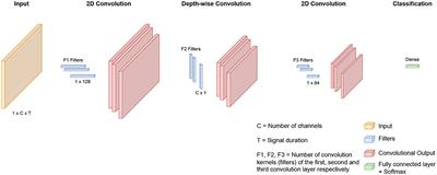
3.3 Backbone network

In this study, we proposed a feature extraction network to analyze sleep EEG signals. The network consists of two main components: a convolutional neural network (SleepNet) and a multilayer transformer encoder module. Which is shown in Figure 4 and Stage B in Figure 1. The CNN is used to extract local features from the signals, while the transformer is used to capture global correlations between different parts of the signals.

Figure 4. Backbone network.

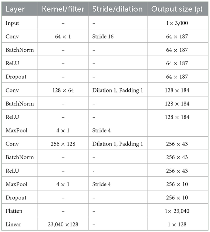
3.3.1 SleepNet features extraction

The CNN component comprises three convolutional layers with batch normalization and dropout, followed by a linear layer, as shown in the Table 1. The first layer has 64 filters with a kernel size of 64 and a stride of 16. The second layer has 128 filters with a kernel size of 8 and a pooling layer with a kernel size of 4. The third layer has 256 filters with a kernel size of 8 and a pooling layer with a kernel size of 4.

Table 1. CNN feature extraction.

Formally, SleeNet extracts the ith feature from one EEG epoch Xi, CNN(θr) represents CNN converted from single channel EEG to eigenvector, and θr is the variable parameter of the CNN. The size of fXi depends on the sampling rate of input EEG. In the formula, f represents the CNN network we use. As shown in the following formula:

f(Xi)=CNN(θr)(Xi),    (12)

the network is trained using the NAdam optimizer to minimize the cross-entropy loss.

3.3.2 Transformer encoder module

The output of the third pooling layer is fed to the transformer component, which consists of encoder layers and transformer encoder. The encoder layer has a dimensionality of 128 and an attention mechanism. The encoder is applied to the input signals, and the output is averaged along the time axis before being fed to a fully connected layer with a 128-dimensional output. After the feedforward layer, our output feature vector is fed into the prototype network. After feature extraction of transformer encoder module, feature output formula is as follows:

F(Xi)=Encoder(f(Xi)),    (13)

where FXi represents features extracted by CNN and Transformer.

3.4 Model settings

Before using a prototypical network, we need to extract features from the collected data. We can construct a prototypical network architecture with five-way (1-shot, 3-shot, 5-shot, 10-shot, 15-shot, 20-shot, 25-shot). We randomly select 1, 3, 5, 10, 15, 20, and 25 epochs from the W, N1, N2, N3, and R phases of the meta-training set, respectively. The five sleep phases are preprocessed and SleepNet with transformer is used as our pre-trained neural network to compute prototypes for each sleep phase.

We divided a batch process into a support set and a query set, utilizing the embedding vectors of the support set to establish a class prototype. This prototype represented a typical embedding vector of a given class, and we then utilized values closely related to it for classification to compare the performance of our approach. In our experiment, Cosine distance, Manhattan distance, Euclidean distance, and Chebyshev distance were used as comparisons, and we obtain the Cosine distance as our best matching and most accurate measurement function. As such, we adopted the Cosine distance function as our distance evaluation metric.

To train the backbone network, we use the NAdam optimizer. To learn feature centers for distinct classes, we employ a stochastic gradient descent optimizer with a learning rate of 0.0009 and a center-loss weight of 0.0009. Among them, we use the pre-trained neural network to extract feature vectors, take the average value, conduct normalization processing, and use softmax for prediction analysis. Experiments were performed on 50 times and then fine-tuned by taking the average loss of gradient descent.

In the meta-testing, the remaining subjects from the meta-training were used as the meta-testing set, as a previously unseen category, for cross-subject EEG sleep staging. We randomly selected N samples in five sleep periods from the meta-testing set, and the five groups of samples were used as the meta-testing support set. Similar to meta-training, after building the initial prototype network on the first layer, we introduced the TDO method, including introducing a high confidence unlabeled query set as our support set, and recalculating the prototype network. All the rest sleep data is used as the meta-testing set, and the construction task is verified repeatedly. The average accuracy is taken as the accuracy of the final test result and the ACC, F1 values, and the accuracy of each category are obtained.

Since the experimental results may vary depending on the chosen support set sample, this experiment is repeated 50 times using the support set randomly, and the average precision is obtained as the final statistical result of the experiment. The average accuracy is taken as the accuracy of the final test result and the ACC, F1 values, and the accuracy of each category are obtained.

3.5 Evaluation

In our experiments, different subjects were used for cross-subject validation for meta-training and meta-testing subjects, and the meta-testing query set did not include meta-training subjects. Our experiments were conducted for 20 rounds, thus validating our experimental results. The experiment is a multi-class classification task for sleep staging. Accuracy, F-measure, recall, and kappa values are used to evaluate the performance of sleep staging. The overall performance is evaluated in terms of accuracy and Cohen's Kappa coefficient. The above evaluation metrics are formulated as follows:

Accuracy=TP+TNTP+FP+TN+FN,    (14) κ=Accu